Abstract

BRGenomics is designed to help users avoid code repetition by providing efficient and tested functions to accomplish common, discrete tasks in the analysis of high-throughput sequencing data. The included functions are geared toward analyzing basepair-resolution sequencing data, the properties of which are exploited to increase performance and user-friendliness. We leverage standard Bioconductor methods and classes to maximize compatability with its rich ecoystem of bioinformatics tools, and we aim to make BRGenomics sufficient for most post-alignment data processing. Common data processing and analytical steps are turned into fast-running one-liners that can be simultaneously applied across numerous datasets. BRGenomics is fully-documented, and we aim it to be beginner-friendly.

Overview

Motivation

This package is designed to:

Replace the use of command-line utilities for most post-alignment processing, e.g. bedtools and deeptools
Be easy-to-use and easy-to-install, without requiring external dependencies, e.g. hitslib or the kent source utilities from the UCSC genome browser
Allow users to string together common analysis pipelines with simple, fast-running one-liners
Avoid code repetition by providing tested and validated code
Exploit the properties of basepair-resolution data to optimize performance and increase user-friendliness
Use process forking to make use of multicore processors
Maximize compatability with Bioconductor’s rich ecosystem of analysis software, in addition to leveraging the traditional strengths of R in statistics and data visualization
Fully replace the bigWig R package

Features

Process and import bedGraph, bigWig, and bam files quickly and easily, with several pre-configured defaults for typical uses
Count and filter spike-in reads
Calculate spike-in normalization factors using several methods and options, including options for batch normalization
Count reads by regions of interest
Count reads at positions within regions of interest, at single-base resolution or in larger bins, and generate count matrices for heatmapping
Calculate bootstrapped signal (e.g. readcount) profiles with confidence intervals (i.e. meta-profiles)
Modify gene regions (e.g. extract promoters or genebody regions) using a single simple and straightforward function
Conveniently and efficiently call DESeq2 to calculate differential expression in a manner that is robust to global changes¹
- Use non-contiguous genes in DESeq2 analysis, e.g. to exclude of specific sites/peaks from the analysis (not usually supported by DESeq2)
- Efficiently generate results across a list of comparisons
Support for blacklisting throughout, and proper accounting of blacklisted sites in relevant calculations
Users interact with an intuitive and computationally efficient data structure (the “basepair resolution GRanges” object), which is already supported by a rich, user-friendly suite of tools that greatly simplify working with datasets and annotations

Coming Soon

Data processing:

Summarizing and plotting replicate correlations
Function to use random read sampling to assess if sequencing depth sufficient to stabilize arbitrary calculations (so a user can supply anonymous function to calculate things like rank expression, power analysis or differential expression by DESeq2, pausing indices, etc.)

Signal counting and analysis:

Two-stranded meta-profile calculations
Automated generation of a list of DESeq2 comparisons using all possible combinations; all possible permutations; or by defining a simple hierarchy of each-vs-one comparisons

Getting started

Installation

As of Bioconductor 3.11 (release date April 28, 2020), BRGenomics can be installed directly from Bioconductor:

# install.packages("BiocManager")
BiocManager::install("BRGenomics")

## Bioconductor version 3.11 (BiocManager 1.30.10), R Under development (unstable)
##   (2020-01-10 r77651)

## Installing package(s) 'BRGenomics'

## Warning: package 'BRGenomics' is not available (for R Under development)

## Warning: unable to access index for repository https://cran.rstudio.com/bin/macosx/el-capitan/contrib/4.0:
##   cannot open URL 'https://cran.rstudio.com/bin/macosx/el-capitan/contrib/4.0/PACKAGES'

## Old packages: 'AnnotationHub', 'backports', 'BiocCheck', 'BiocGenerics',
##   'biocViews', 'biomaRt', 'Biostrings', 'callr', 'class', 'ComplexHeatmap',
##   'cytolib', 'DelayedArray', 'DT', 'factoextra', 'flowCore', 'flowWorkspace',
##   'foreach', 'foreign', 'fs', 'gdtools', 'GenomeInfoDb', 'GenomicAlignments',
##   'GenomicFiles', 'GenomicRanges', 'GGally', 'ggplot2', 'glue', 'gtools',
##   'Hmisc', 'IRanges', 'lattice', 'lemon', 'lme4', 'locfit', 'lubridate',
##   'ncdfFlow', 'pkgdown', 'poweRlaw', 'quantreg', 'Rcpp', 'regioneR',
##   'rematch2', 'reticulate', 'robustbase', 'RProtoBufLib', 'S4Vectors',
##   'SummarizedExperiment', 'tibble', 'tinytex', 'usethis', 'xml2', 'XVector'

Alternatively, the latest development version can be installed from
GitHub:

# install.packages("remotes")
remotes::install_github("mdeber/BRGenomics@R3")

BRGenomics (and Bioconductor 3.11) require R version 4.0 (release April 24, 2020). Installing the R3 branch, as shown above, is required to install under R 3.x.

If you install the development version from Github and you’re using Windows, Rtools for Windows is required.

Parallel Processing

By default, many BRGenomics functions use multicore processing as implemented in the parallel package. BRGenomics functions that can be parallelized always contain the argument ncores. If not specified, the default is to use the global option “mc.cores” (the same option used by the parallel package), or 2 if that option is not set.

If you wanted to change the global default to 4 cores, for example, you would run options(mc.cores = 4) at the start of your R session. If you’re unsure how many cores your processor has, run parallel::detectCores().

While performance can be memory constrained in some cases (and thus actually hampered by excessive parallelization), substantial performance benefits can be acheived by maximizing parallelization.

However, parallel processing is not available on Windows. To maintain compatability, all code in this vignette as well as the example code in the documentation is to use a single core, i.e. ncores = 1.

Included Datasets

BRGenomics ships with an example dataset of PRO-seq data from Drosophila melanogaster². PRO-seq is a basepair-resolution method that uses 3’-end sequencing of nascent RNA to map the locations of actively engaged RNA polymerases.

To keep the dataset small, we’ve only included reads mapping to the fourth chromosome³.

The included datasets can be accessed using the data() function:

library(BRGenomics)

data("PROseq")
PROseq

## GRanges object with 47380 ranges and 1 metadata column:
##           seqnames    ranges strand |     score
##              <Rle> <IRanges>  <Rle> | <integer>
##       [1]     chr4      1295      + |         1
##       [2]     chr4     41428      + |         1
##       [3]     chr4     42588      + |         1
##       [4]     chr4     42590      + |         2
##       [5]     chr4     42593      + |         5
##       ...      ...       ...    ... .       ...
##   [47376]     chr4   1307742      - |         1
##   [47377]     chr4   1316537      - |         1
##   [47378]     chr4   1318960      - |         1
##   [47379]     chr4   1319004      - |         1
##   [47380]     chr4   1319369      - |         1
##   -------
##   seqinfo: 7 sequences from an unspecified genome

Notice that the data is contained within a GRanges object. GRanges objects, from the GenomicRanges package, are very easy to work with, and are supported by a plethora of useful functions and packages.

The structure of the data will be described later on (in section “Basepair-Resolution GRanges Objects”). For now, we’ll just note that both annotations (e.g. genelists) and data are contained using the same GRanges class.

We’ve included an example genelist to accompany the PRO-seq data:

data("txs_dm6_chr4")
txs_dm6_chr4

## GRanges object with 339 ranges and 2 metadata columns:
##         seqnames          ranges strand |     tx_name     gene_id
##            <Rle>       <IRanges>  <Rle> | <character> <character>
##     [1]     chr4        879-5039      + | FBtr0346692 FBgn0267363
##     [2]     chr4     42774-43374      + | FBtr0344900 FBgn0266617
##     [3]     chr4     44774-46074      + | FBtr0340499 FBgn0265633
##     [4]     chr4     56497-60974      + | FBtr0333704 FBgn0264617
##     [5]     chr4     56497-63124      + | FBtr0333705 FBgn0264617
##     ...      ...             ...    ... .         ...         ...
##   [335]     chr4 1192419-1196848      - | FBtr0100543 FBgn0039924
##   [336]     chr4 1192419-1196848      - | FBtr0100544 FBgn0039924
##   [337]     chr4 1225089-1230713      - | FBtr0100406 FBgn0027101
##   [338]     chr4 1225737-1230713      - | FBtr0100402 FBgn0027101
##   [339]     chr4 1225737-1230713      - | FBtr0100404 FBgn0027101
##   -------
##   seqinfo: 7 sequences from dm6 genome

The GRanges above contains all Flybase annotated transcripts from chromosome 4, with no filtering of any kind.

Basic Operations on GRanges

For users who are unfamiliar with GRanges objects, this section demonstrates a number of basic operations.

A quick summary of the general strcture: Each element of a GRanges object is called a “range”. As you can see above, each range consists of several components: seqnames, ranges, and strand. These essential attributes are all found to the left of the vertical divider above; everything to the right of that divider is an optional, metadata attribute.

The core attributes can be accessed using the functions seqnames(), ranges(), and strand(). All metadata can be accessed using mcols(), and individual columns are accessable with the $ operator. The only reserved metadata column is the score column, which is just like any other metadata column, except that users can use the score() function to assess it.

All of the above functions are both “getters” and “setters”, e.g. strand(x) returns the strand information, and strand(x) <- "+" assigns it.

These and other operations are demonstrated below.

To learn more about GRanges objects, including a general overview of their components, see the useful vignette An Introduction to the GenomicRanges Package. Alternatively, see the archived materials from the 2018 Bioconductor workshop Solving Common Bioinformatic Challenges Using GenomicRanges. Note that this package will implement and streamline a number of common operations, but users should still have a basic familiarity with GRanges objects.

Get the length of the genelist:

length(txs_dm6_chr4)

## [1] 339

Select the 2nd transcript:

txs_dm6_chr4[2]

## GRanges object with 1 range and 2 metadata columns:
##       seqnames      ranges strand |     tx_name     gene_id
##          <Rle>   <IRanges>  <Rle> | <character> <character>
##   [1]     chr4 42774-43374      + | FBtr0344900 FBgn0266617
##   -------
##   seqinfo: 7 sequences from dm6 genome

Select 4 transcipts:

tx4 <- txs_dm6_chr4[c(1, 10, 200, 300)]
tx4

## GRanges object with 4 ranges and 2 metadata columns:
##       seqnames          ranges strand |     tx_name     gene_id
##          <Rle>       <IRanges>  <Rle> | <character> <character>
##   [1]     chr4        879-5039      + | FBtr0346692 FBgn0267363
##   [2]     chr4    69326-110059      + | FBtr0308615 FBgn0085432
##   [3]     chr4   184225-193489      - | FBtr0089150 FBgn0039890
##   [4]     chr4 1009895-1027101      - | FBtr0309865 FBgn0025741
##   -------
##   seqinfo: 7 sequences from dm6 genome

Get the lengths of the first 4 transcripts:

width(tx4)

## [1]  4161 40734  9265 17207

Get a dataframe of the metadata for the first 4 transcripts:

mcols(tx4)

## DataFrame with 4 rows and 2 columns
##       tx_name     gene_id
##   <character> <character>
## 1 FBtr0346692 FBgn0267363
## 2 FBtr0308615 FBgn0085432
## 3 FBtr0089150 FBgn0039890
## 4 FBtr0309865 FBgn0025741

Access a single metadata column for the first 4 transcripts:

mcols(tx4)[, 2]

## [1] "FBgn0267363" "FBgn0085432" "FBgn0039890" "FBgn0025741"

mcols(tx4)[, "gene_id"]

## [1] "FBgn0267363" "FBgn0085432" "FBgn0039890" "FBgn0025741"

tx4$gene_id

## [1] "FBgn0267363" "FBgn0085432" "FBgn0039890" "FBgn0025741"

tx4_names <- tx4$tx_name
tx4_names

## [1] "FBtr0346692" "FBtr0308615" "FBtr0089150" "FBtr0309865"

Get the first gene_id (a metadata element):

tx4$gene_id[1]

## [1] "FBgn0267363"

Remove a metadata column:

mcols(tx4) <- mcols(tx4)[, -1]
tx4

## GRanges object with 4 ranges and 1 metadata column:
##       seqnames          ranges strand |           X
##          <Rle>       <IRanges>  <Rle> | <character>
##   [1]     chr4        879-5039      + | FBgn0267363
##   [2]     chr4    69326-110059      + | FBgn0085432
##   [3]     chr4   184225-193489      - | FBgn0039890
##   [4]     chr4 1009895-1027101      - | FBgn0025741
##   -------
##   seqinfo: 7 sequences from dm6 genome

Rename metadata:

names(mcols(tx4)) <- "gene_id"
tx4

## GRanges object with 4 ranges and 1 metadata column:
##       seqnames          ranges strand |     gene_id
##          <Rle>       <IRanges>  <Rle> | <character>
##   [1]     chr4        879-5039      + | FBgn0267363
##   [2]     chr4    69326-110059      + | FBgn0085432
##   [3]     chr4   184225-193489      - | FBgn0039890
##   [4]     chr4 1009895-1027101      - | FBgn0025741
##   -------
##   seqinfo: 7 sequences from dm6 genome

Add metadata; same as access methods (mcols()[], mcols()$, or simply $):

tx4$tx_name <- tx4_names
tx4

## GRanges object with 4 ranges and 2 metadata columns:
##       seqnames          ranges strand |     gene_id     tx_name
##          <Rle>       <IRanges>  <Rle> | <character> <character>
##   [1]     chr4        879-5039      + | FBgn0267363 FBtr0346692
##   [2]     chr4    69326-110059      + | FBgn0085432 FBtr0308615
##   [3]     chr4   184225-193489      - | FBgn0039890 FBtr0089150
##   [4]     chr4 1009895-1027101      - | FBgn0025741 FBtr0309865
##   -------
##   seqinfo: 7 sequences from dm6 genome

Modify metadata:

tx4$gene_id[1] <- "gene1"
tx4$tx_name <- 1:4
tx4

## GRanges object with 4 ranges and 2 metadata columns:
##       seqnames          ranges strand |     gene_id   tx_name
##          <Rle>       <IRanges>  <Rle> | <character> <integer>
##   [1]     chr4        879-5039      + |       gene1         1
##   [2]     chr4    69326-110059      + | FBgn0085432         2
##   [3]     chr4   184225-193489      - | FBgn0039890         3
##   [4]     chr4 1009895-1027101      - | FBgn0025741         4
##   -------
##   seqinfo: 7 sequences from dm6 genome

Get beginning of ranges (not strand specific):

start(tx4)

## [1]     879   69326  184225 1009895

Get beginning of ranges (strand specific):

tx4_tss <- resize(tx4, width = 1, fix = "start")
tx4_tss

## GRanges object with 4 ranges and 2 metadata columns:
##       seqnames    ranges strand |     gene_id   tx_name
##          <Rle> <IRanges>  <Rle> | <character> <integer>
##   [1]     chr4       879      + |       gene1         1
##   [2]     chr4     69326      + | FBgn0085432         2
##   [3]     chr4    193489      - | FBgn0039890         3
##   [4]     chr4   1027101      - | FBgn0025741         4
##   -------
##   seqinfo: 7 sequences from dm6 genome

start(tx4_tss)

## [1]     879   69326  193489 1027101

Remove all metadata:

mcols(tx4) <- NULL
tx4

## GRanges object with 4 ranges and 0 metadata columns:
##       seqnames          ranges strand
##          <Rle>       <IRanges>  <Rle>
##   [1]     chr4        879-5039      +
##   [2]     chr4    69326-110059      +
##   [3]     chr4   184225-193489      -
##   [4]     chr4 1009895-1027101      -
##   -------
##   seqinfo: 7 sequences from dm6 genome

Importing & Modifying Genelists

Importing Annotations with rtracklayer

Importing genomics files is accomplished using the rtracklayer package, which contains a variety of functions and options for importing and exporting.

# import bed file
genelist <- import.bed("~/data/genelists/genes.bed")

# import gff
genelist <- import.gff("~/data/genelists/genes.gff")

# export a bed file after modifying
export.bed(genelist, "~/data/genelists/filtered_genes.bed")

Defining Regions Using the genebodies Function

One of the more useful GenomicRanges functions is the promoters function, which returns ranges centered on the strand-specific start of the input ranges:

data("txs_dm6_chr4")
tx4 <- txs_dm6_chr4[c(1, 10, 200, 300)]
tx4

## GRanges object with 4 ranges and 2 metadata columns:
##       seqnames          ranges strand |     tx_name     gene_id
##          <Rle>       <IRanges>  <Rle> | <character> <character>
##   [1]     chr4        879-5039      + | FBtr0346692 FBgn0267363
##   [2]     chr4    69326-110059      + | FBtr0308615 FBgn0085432
##   [3]     chr4   184225-193489      - | FBtr0089150 FBgn0039890
##   [4]     chr4 1009895-1027101      - | FBtr0309865 FBgn0025741
##   -------
##   seqinfo: 7 sequences from dm6 genome

tx4_pr <- promoters(tx4, upstream = 50, downstream = 100)
tx4_pr

## GRanges object with 4 ranges and 2 metadata columns:
##       seqnames          ranges strand |     tx_name     gene_id
##          <Rle>       <IRanges>  <Rle> | <character> <character>
##   [1]     chr4         829-978      + | FBtr0346692 FBgn0267363
##   [2]     chr4     69276-69425      + | FBtr0308615 FBgn0085432
##   [3]     chr4   193390-193539      - | FBtr0089150 FBgn0039890
##   [4]     chr4 1027002-1027151      - | FBtr0309865 FBgn0025741
##   -------
##   seqinfo: 7 sequences from dm6 genome

width(tx4_pr)

## [1] 150 150 150 150

BRGenomics ships with a more flexible alternative function called genebodies. While promoters has the arguments upstream and downstream, which take only positive values, the genebodies function uses start and end arguments that can be positive or negative, and arguments fix.start and fix.end for determining whether to define the positions in relation to the (strand-specific) beginning or ends of genes.

Below, we demonstrate several uses of the genebodies function, using a list of transcripts which start at a transcription start site (TSS) and end at a cleavage and polyadenylation site (CPS).

Original regions:

tx4

## GRanges object with 4 ranges and 2 metadata columns:
##       seqnames          ranges strand |     tx_name     gene_id
##          <Rle>       <IRanges>  <Rle> | <character> <character>
##   [1]     chr4        879-5039      + | FBtr0346692 FBgn0267363
##   [2]     chr4    69326-110059      + | FBtr0308615 FBgn0085432
##   [3]     chr4   184225-193489      - | FBtr0089150 FBgn0039890
##   [4]     chr4 1009895-1027101      - | FBtr0309865 FBgn0025741
##   -------
##   seqinfo: 7 sequences from dm6 genome

Genebody regions from 300 bp downstream of the TSS to 300 bp upstream of the CPS:

genebodies(tx4, start = 300, end = -300)

## GRanges object with 4 ranges and 2 metadata columns:
##       seqnames          ranges strand |     tx_name     gene_id
##          <Rle>       <IRanges>  <Rle> | <character> <character>
##   [1]     chr4       1179-4739      + | FBtr0346692 FBgn0267363
##   [2]     chr4    69626-109759      + | FBtr0308615 FBgn0085432
##   [3]     chr4   184525-193189      - | FBtr0089150 FBgn0039890
##   [4]     chr4 1010195-1026801      - | FBtr0309865 FBgn0025741
##   -------
##   seqinfo: 7 sequences from dm6 genome

By default, fix.start = "start" and fix.end = "end". But we can change either of them to define ranges based solely on the beginnings or ends of the input regions.

Get promoter regions from 50 bp upstream to 100 bp downstream of the TSS:

genebodies(tx4, -50, 100, fix.end = "start")

## GRanges object with 4 ranges and 2 metadata columns:
##       seqnames          ranges strand |     tx_name     gene_id
##          <Rle>       <IRanges>  <Rle> | <character> <character>
##   [1]     chr4         829-979      + | FBtr0346692 FBgn0267363
##   [2]     chr4     69276-69426      + | FBtr0308615 FBgn0085432
##   [3]     chr4   193389-193539      - | FBtr0089150 FBgn0039890
##   [4]     chr4 1027001-1027151      - | FBtr0309865 FBgn0025741
##   -------
##   seqinfo: 7 sequences from dm6 genome

Regions from 100 bp upstream of to 50 bp upstream of the TSS:

genebodies(tx4, -100, -50, fix.end = "start")

## GRanges object with 4 ranges and 2 metadata columns:
##       seqnames          ranges strand |     tx_name     gene_id
##          <Rle>       <IRanges>  <Rle> | <character> <character>
##   [1]     chr4         779-829      + | FBtr0346692 FBgn0267363
##   [2]     chr4     69226-69276      + | FBtr0308615 FBgn0085432
##   [3]     chr4   193539-193589      - | FBtr0089150 FBgn0039890
##   [4]     chr4 1027151-1027201      - | FBtr0309865 FBgn0025741
##   -------
##   seqinfo: 7 sequences from dm6 genome

Regions from 1kb upstream of the CPS to 1kb downstream of the CPS

genebodies(tx4, -1000, 1000, fix.start = "end")

## GRanges object with 4 ranges and 2 metadata columns:
##       seqnames          ranges strand |     tx_name     gene_id
##          <Rle>       <IRanges>  <Rle> | <character> <character>
##   [1]     chr4       4039-6039      + | FBtr0346692 FBgn0267363
##   [2]     chr4   109059-111059      + | FBtr0308615 FBgn0085432
##   [3]     chr4   183225-185225      - | FBtr0089150 FBgn0039890
##   [4]     chr4 1008895-1010895      - | FBtr0309865 FBgn0025741
##   -------
##   seqinfo: 7 sequences from dm6 genome

Regions within the first 10kb downstream of the CPS:

genebodies(tx4, 0, 10000, fix.start = "end")

## GRanges object with 4 ranges and 2 metadata columns:
##       seqnames         ranges strand |     tx_name     gene_id
##          <Rle>      <IRanges>  <Rle> | <character> <character>
##   [1]     chr4     5039-15039      + | FBtr0346692 FBgn0267363
##   [2]     chr4  110059-120059      + | FBtr0308615 FBgn0085432
##   [3]     chr4  174225-184225      - | FBtr0089150 FBgn0039890
##   [4]     chr4 999895-1009895      - | FBtr0309865 FBgn0025741
##   -------
##   seqinfo: 7 sequences from dm6 genome

Basepair-Resolution GRanges Objects

Let’s examine the included PRO-seq data:

data("PROseq")
PROseq

## GRanges object with 47380 ranges and 1 metadata column:
##           seqnames    ranges strand |     score
##              <Rle> <IRanges>  <Rle> | <integer>
##       [1]     chr4      1295      + |         1
##       [2]     chr4     41428      + |         1
##       [3]     chr4     42588      + |         1
##       [4]     chr4     42590      + |         2
##       [5]     chr4     42593      + |         5
##       ...      ...       ...    ... .       ...
##   [47376]     chr4   1307742      - |         1
##   [47377]     chr4   1316537      - |         1
##   [47378]     chr4   1318960      - |         1
##   [47379]     chr4   1319004      - |         1
##   [47380]     chr4   1319369      - |         1
##   -------
##   seqinfo: 7 sequences from an unspecified genome

This GRanges object is constructed such that each range has a width of 1 (i.e. each range represents a single base in the genome), and each range has an associated score, which contains signal information for that base.

We refer to a GRanges object formatted in this way as a basepair-resolution GRanges object⁴, and this structure underpins much of BRGenomics.

In the included PRO-seq data, the positional information is determined by the 3’ end of mapped reads, and the signal information is the number of reads containing that 3’ end.

bigWig files, as well as coverage objects in GenomicRanges, use a form of compression in which adjacent positions sharing the same signal are combined. For whole-read coverage methods, this run-length encoding enhances performance and efficiency. However, basepair resolution data is not nearly as smooth, and its rare that adjacent bases share the same signal. With basepair resolution data, combining adjacent positions increases complexity, while providing a negligible storage benefit.

Splitting up each base into its own range (its own index) results in a number of downstream computational benefits. Perhaps more importantly, however, is the added simplicity for the user: each index of a basepair-resolution GRanges object addresses a single genomic position and its associated signal.

length(PROseq) # number of unique positions in dataset
## [1] 47380
sum(score(PROseq)) # total number of reads
## [1] 73887
sum(score(PROseq) == 1) # number of sites with only a single read
## [1] 37559

subset(PROseq, score > 10) # sites with more than 10 reads

## GRanges object with 309 ranges and 1 metadata column:
##         seqnames    ranges strand |     score
##            <Rle> <IRanges>  <Rle> | <integer>
##     [1]     chr4     69377      + |        12
##     [2]     chr4     69391      + |        12
##     [3]     chr4     69397      + |        25
##     [4]     chr4     69401      + |       122
##     [5]     chr4     69692      + |        17
##     ...      ...       ...    ... .       ...
##   [305]     chr4   1176185      - |        13
##   [306]     chr4   1182428      - |        52
##   [307]     chr4   1196793      - |        54
##   [308]     chr4   1196794      - |        14
##   [309]     chr4   1226558      - |        13
##   -------
##   seqinfo: 7 sequences from an unspecified genome

We can write a simple test to determine if a GRanges object is “basepair-resolution”: all ranges have widths of 1, and no position is duplicated.

all(width(PROseq) == 1)
## [1] TRUE
isDisjoint(PROseq) # [*]
## [1] TRUE

[*] A “disjoint” GRanges is one in which none of the ranges overlap one another.

For convenience, we’ve included a test function:

isBRG(PROseq)

## [1] TRUE

The page on Importing and Processing Data also serves to emphasize the characteristics of the basepair-resolution GRanges object, and demonstrates some alternatives that can be used within this pacakge.

When to use “Basepair-Resolution” Objects

The reason single-base ranges are efficient for true, basepair-resolution data is that it’s generally uncommon for adjacent positions to have the same signal.

However, for most other kinds of data, e.g. whole-read coverage data or smoothed/imputed data, it’s very common for strings of identical values to be present.

For non-basepair-resolution data (non-“spikey” data), be sure to import data using the argument makeBRG = FALSE, and look for functions that contain an expand_ranges argument and set it to TRUE.

If expand_ranges = FALSE, functions will assume that any range spanning multiple positions represents a single molecule (or type of molecule) that spans exactly those positions, e.g. a range covering 30 bases with score = 2 represents two identical reads. When expand_ranges = TRUE, that same range will be treated as 60 “reads” (or signal values).

Internally, BRGenomics deals with non-basepair-resolution ranges in a much more efficient manner than explicitly expanding them.

Importing and Processing Data

BRGenomics provides several functions for conveniently importing and processing BAM, bigWig, bedGraph files.

Importing BAM Files

The import_bam function provides a number of options for filtering and processing bam files. BRGenomics includes an example BAM file with a small number of reads from the included PRO-seq data. The file’s local location can be found (on your computer) as follows:

bfile <- system.file("extdata", "PROseq_dm6_chr4.bam", 
                     package = "BRGenomics")

Because PRO-seq data is sequenced in the 3’-to-5’ direction of the original RNA molecule, we’ll use the revcomp option to reverse-complement all the input reads. We’ll also set a minimum MAPQ score of 20:

ps_reads <- import_bam(bfile, mapq = 20, revcomp = TRUE, paired_end = FALSE)
ps_reads

## GRanges object with 164 ranges and 1 metadata column:
##         seqnames          ranges strand |     score
##            <Rle>       <IRanges>  <Rle> | <integer>
##     [1]     chr4       1270-1296      + |         1
##     [2]     chr4     41411-41429      + |         1
##     [3]     chr4     42556-42591      + |         1
##     [4]     chr4     42559-42589      + |         1
##     [5]     chr4     42559-42594      + |         3
##     ...      ...             ...    ... .       ...
##   [160]     chr4 1307741-1307776      - |         1
##   [161]     chr4 1316536-1316563      - |         1
##   [162]     chr4 1318959-1318994      - |         1
##   [163]     chr4 1319003-1319038      - |         1
##   [164]     chr4 1319368-1319403      - |         1
##   -------
##   seqinfo: 1870 sequences from an unspecified genome

By default, import_bam combines identical reads into the same range, and the score metadata column indicatea the number of perfectly-overlapping alignments. This means that the total number of alignments (reads) is equal to the sum of the score:

sum(score(ps_reads))

## [1] 190

Alternatively, you can import each read as its own range by setting field = NULL:

reads_expanded <- import_bam(bfile, mapq = 20, revcomp = TRUE, 
                             field = NULL, paired_end = FALSE)
ps_reads[1:8]

## GRanges object with 8 ranges and 1 metadata column:
##       seqnames      ranges strand |     score
##          <Rle>   <IRanges>  <Rle> | <integer>
##   [1]     chr4   1270-1296      + |         1
##   [2]     chr4 41411-41429      + |         1
##   [3]     chr4 42556-42591      + |         1
##   [4]     chr4 42559-42589      + |         1
##   [5]     chr4 42559-42594      + |         3
##   [6]     chr4 42560-42594      + |         2
##   [7]     chr4 42560-42595      + |         2
##   [8]     chr4 42561-42596      + |         1
##   -------
##   seqinfo: 1870 sequences from an unspecified genome

reads_expanded[1:8]

## GRanges object with 8 ranges and 0 metadata columns:
##       seqnames      ranges strand
##          <Rle>   <IRanges>  <Rle>
##   [1]     chr4   1270-1296      +
##   [2]     chr4 41411-41429      +
##   [3]     chr4 42556-42591      +
##   [4]     chr4 42559-42589      +
##   [5]     chr4 42559-42594      +
##   [6]     chr4 42559-42594      +
##   [7]     chr4 42559-42594      +
##   [8]     chr4 42560-42594      +
##   -------
##   seqinfo: 1870 sequences from an unspecified genome

Notice that reads 5-7 are now identical, rather than combined into a single range with a score = 3.

length(reads_expanded) == sum(score(ps_reads))

## [1] TRUE

Many BRGenomics function have a field argument, and setting field = NULL will treat each range has a single read.

Example: Importing PRO-seq BAM files at Basepair Resolution

We can use the import_bam function to extract the positions of interest from BAM files. Below, we construct an import function for PRO-seq data that returns a basepair-resolution GRanges object.

In PRO-seq, a “run-on” reaction is performed in which actively engaged RNA polymerases incorporate a biotinylated nucleotide at the 3’ end of a nascent RNA. Our base of interest is therefore the base immediately preceding the RNA 3’ end, as this was the original position of a polymerase active site.

The processing options in import_bam are applied in the same order that they’re listed in the documentation page. Following this order, we will apply the options:

Filter reads by a minimum MAPQ score
Take the reverse complement
Shift reads upstream by 1 base
Extract the 3’ base

ps <- import_bam(bfile, 
                 mapq = 20, 
                 revcomp = TRUE,
                 shift = -1,
                 trim.to = "3p",
                 paired_end = FALSE)
ps

## GRanges object with 150 ranges and 1 metadata column:
##         seqnames    ranges strand |     score
##            <Rle> <IRanges>  <Rle> | <integer>
##     [1]     chr4      1295      + |         1
##     [2]     chr4     41428      + |         1
##     [3]     chr4     42588      + |         1
##     [4]     chr4     42590      + |         2
##     [5]     chr4     42593      + |         5
##     ...      ...       ...    ... .       ...
##   [146]     chr4   1307742      - |         1
##   [147]     chr4   1316537      - |         1
##   [148]     chr4   1318960      - |         1
##   [149]     chr4   1319004      - |         1
##   [150]     chr4   1319369      - |         1
##   -------
##   seqinfo: 1870 sequences from an unspecified genome

Note that for paired-end data, import_bam will automatically filter unmatched read pairs.

Notice that the number of ranges in ps is not the same as for ps_reads, in which we imported the entire read lengths:

length(ps_reads)
## [1] 164
length(ps)
## [1] 150

This is because identical positions are collapsed together after applying the processing options. However, we can check that all of the same reads are represented:

sum(score(ps)) == sum(score(ps_reads))
## [1] TRUE

And we can check that collapsing identical positions has created a basepair-resolution GRanges object:

isBRG(ps)
## [1] TRUE

Pre-formatted Input Functions

For convenience, we’ve included several functions with default options for several kinds of data, including import_bam_PROseq, import_bam_PROcap, and import_bam_ATACseq, the latter of which corrects for the 9 bp offset between Tn5 insertion sites.⁵

Performance Considerations

For single-ended bam files, import is much faster if the bam files are sorted and indexed (i.e. by samtools index).

For paired-end files, we assume that collating (samtools collate) or sorting by name is faster.

Additionally, while single-ended files can often be imported “all at once” (particularly if sorted and indexed), processing paired-end data is more memory intensive, and requires breaking up the file into chunks for processing. For this, use the yieldSize argument.

For example, to process 500 thousands reads at a time, set the yieldSize = 5e5.

Example: Converting BAMs to bigWigs

In conjunction with export functions from the rtracklayer package, we can use the functions described above to write a post-alignment pipeline for generating bigWig files for PRO-seq data:

# import bam, automatically applying processing steps for PRO-seq
ps <- import_bam_PROseq(bfile, mapq = 30, paired_end = FALSE)

# separate strands, and make minus-strand scores negative
ps_plus <- subset(ps, strand == "+")
ps_minus <- subset(ps, strand == "-")
score(ps_minus) <- -score(ps_minus)

# use rtracklayer to export bigWig files
export.bw(ps_plus, "~/Data/PROseq_plus.bw")
export.bw(ps_minus, "~/Data/PROseq_minus.bw")

Importing bedGraphs and bigWigs

bedGraph and bigWig files are efficient and portable, but unstranded representations of basepair-resolution genomics data.

As compared to rtracklayer::import.bedGraph, the BRGenomics function import_bedGraph imports both plus-strand and minus-strand files as a single object, and has options for filtering out odd chromosomes, mitochondrial chromosomes, and sex chromosomes.

# local paths to included bedGraph files
bg.p <- system.file("extdata", "PROseq_dm6_chr4_plus.bedGraph",
                    package = "BRGenomics")
bg.m <- system.file("extdata", "PROseq_dm6_chr4_minus.bedGraph",
                    package = "BRGenomics")

import_bedGraph(bg.p, bg.m, genome = "dm6")

## GRanges object with 164 ranges and 1 metadata column:
##         seqnames          ranges strand |     score
##            <Rle>       <IRanges>  <Rle> | <integer>
##     [1]     chr4       1270-1295      + |         1
##     [2]     chr4     41411-41428      + |         1
##     [3]     chr4     42556-42590      + |         1
##     [4]     chr4     42559-42588      + |         1
##     [5]     chr4     42559-42593      + |         3
##     ...      ...             ...    ... .       ...
##   [160]     chr4 1307742-1307776      - |         1
##   [161]     chr4 1316537-1316563      - |         1
##   [162]     chr4 1318960-1318994      - |         1
##   [163]     chr4 1319004-1319038      - |         1
##   [164]     chr4 1319369-1319403      - |         1
##   -------
##   seqinfo: 1 sequence from dm6 genome; no seqlengths

The import_bigWig function provides the same added functionality as compared to rtracklayer::import.bw, but also removes run-length compression and returns a basepair-resolution GRanges object by default.

# local paths to included bigWig files
bw.p <- system.file("extdata", "PROseq_dm6_chr4_plus.bw",
                    package = "BRGenomics")
bw.m <- system.file("extdata", "PROseq_dm6_chr4_minus.bw",
                    package = "BRGenomics")

import_bigWig(bw.p, bw.m, genome = "dm6")

## GRanges object with 150 ranges and 1 metadata column:
##         seqnames    ranges strand |     score
##            <Rle> <IRanges>  <Rle> | <integer>
##     [1]     chr4      1295      + |         1
##     [2]     chr4     41428      + |         1
##     [3]     chr4     42588      + |         1
##     [4]     chr4     42590      + |         2
##     [5]     chr4     42593      + |         5
##     ...      ...       ...    ... .       ...
##   [146]     chr4   1307742      - |         1
##   [147]     chr4   1316537      - |         1
##   [148]     chr4   1318960      - |         1
##   [149]     chr4   1319004      - |         1
##   [150]     chr4   1319369      - |         1
##   -------
##   seqinfo: 1 sequence from dm6 genome

Conversion to a basepair-resolution GRanges object can be turned off by setting makeBRG = FALSE.

Signal Counting

Signal by Region

The getCountsByRegion function counts signal within regions of interest, and returns a simple vector.

library(BRGenomics)
data("PROseq")
data("txs_dm6_chr4")

counts_txs <- getCountsByRegions(PROseq, txs_dm6_chr4)
counts_txs[1:5]
## [1]   1  59  13 126 263
length(txs_dm6_chr4) == length(counts_txs)
## [1] TRUE

Signal by Position and Region

The getCountsByPositions function will count signal at each position within each region of interest. By default, a matrix is returned, with a row for each region, and a column for each position.

# get first 100 bases of each transcript
txs_pr <- promoters(txs_dm6_chr4, 0, 100)
# get signal at each base within each promoter region
countmatrix_pr <- getCountsByPositions(PROseq, txs_pr)

class(countmatrix_pr)
## [1] "matrix"
nrow(countmatrix_pr) == length(txs_pr)
## [1] TRUE
ncol(countmatrix_pr) == width(txs_pr[1])
## [1] TRUE

By default, each “position” (each column) is a single base, but counting can be done in bins as well:

# get signal in 10 bp bins within each promoter region
countmatrix_pr_bin <- getCountsByPositions(PROseq, txs_pr, binsize = 10)
countmatrix_pr_bin[1:5, ]

##      [,1] [,2] [,3] [,4] [,5] [,6] [,7] [,8] [,9] [,10]
## [1,]    0    0    0    0    0    0    0    0    0     0
## [2,]    2    1    7    1    0    0    0    3    2     0
## [3,]    0    0    1    0    0    0    1    0    0     0
## [4,]    0    0    0    0    0    0    0    0    0     0
## [5,]    0    0    0    0    0    0    0    0    0     0

all(rowSums(countmatrix_pr_bin) == rowSums(countmatrix_pr))
## [1] TRUE

By default, an error is returned if input regions aren’t all the same size:

getCountsByPositions(PROseq, txs_dm6_chr4)

## Error in .get_cbp_mw(hits, dataset.gr, regions.gr, binsize, FUN, smw, : regions.gr contains ranges with multiple widths, but simplify.multi.widths is set to 'error'. Did you mean to call getCountsByRegions instead?

This is intended to avoid accidental use of getCountsByPositions in lieu of getCountsByRegions. However, for the rare case when users do intend to use multi-width regions, there is support for this using the simplify.multi.widths argument, which contains several useful options for how to do this (see the documentation for more details).

Example: Plot Signal Over a Gene

We can use getCountsByPositions to get the signal profile over a single gene. Let’s have a look at the gene with the highest signal near the TSS:

idx <- which.max(rowSums(countmatrix_pr))
idx
## [1] 135

plot(x = 1:ncol(countmatrix_pr), 
     y = countmatrix_pr[idx, ], 
     type = "h", 
     main = txs_pr$tx_name[idx],
     xlab = "Distance to TSS",
     ylab = "PRO-seq Signal")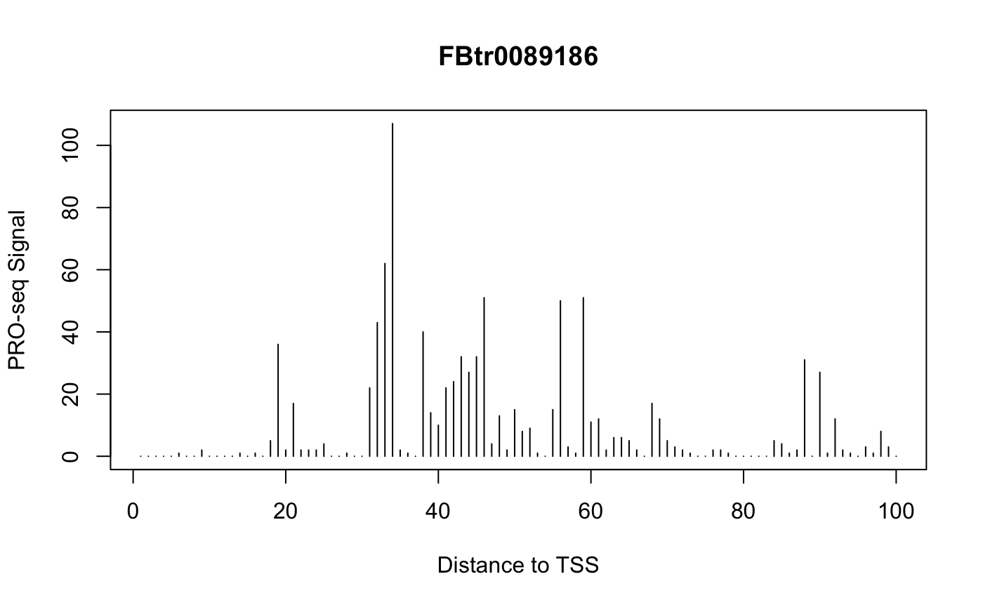

Example: Plot Signal Heatmap

A typical use of getCountsByPositions is to generate a heatmap of signal by position within a list of genes. The ComplexHeatmap package is well documented and offers a high level of functionality, but we can also use ggplot2 to generate customizable heatmaps.

To format our matrix for ggplot, we want to “melt” it. The package reshape2 can melt matrices into dataframes, but BRGenomics also provides a melt argument for several functions, including getCountsByPositions:

cbp.df <- getCountsByPositions(PROseq, txs_pr, binsize = 10, 
                               melt = TRUE, ncores = 1)
head(cbp.df)

##   region position signal
## 1      1        1      0
## 2      1        2      0
## 3      1        3      0
## 4      1        4      0
## 5      1        5      0
## 6      1        6      0

As you can see, the rows and columns of the matrix are now described in columns of this dataframe, and the signal held at each position is in the third column. Now we can plot:

library(ggplot2)

ggplot(cbp.df, aes(x = 10*position - 5, y = region, fill = signal)) + 
  geom_raster() + 
  coord_cartesian(expand = FALSE) + 
  labs(x = "Distance from TSS", y = "Transcript", 
       title = "PRO-seq", fill = "Reads") + 
  theme_bw()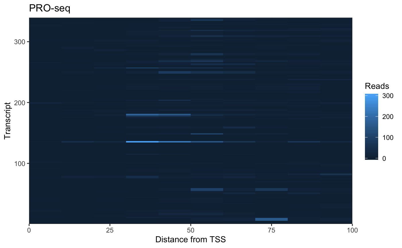

The high dynamic range of PRO-seq data means that regions (rows) with less signal are hard to pick out. To address this, we can row-normalize the data:

rn_cbp <- countmatrix_pr / rowSums(countmatrix_pr)
rn_cbp.df <- reshape2::melt(rn_cbp, varnames = c("region", "position"),
                            value.name = "signal")
ggplot(rn_cbp.df, 
       aes(x = 10*position - 5, y = region, fill = signal)) + 
  geom_raster() + 
  coord_cartesian(expand = FALSE) + 
  labs(x = "Distance from TSS", y = "Transcript", 
       title = "Row-Normalized PRO-seq (%)", fill = "Reads") + 
  theme_bw()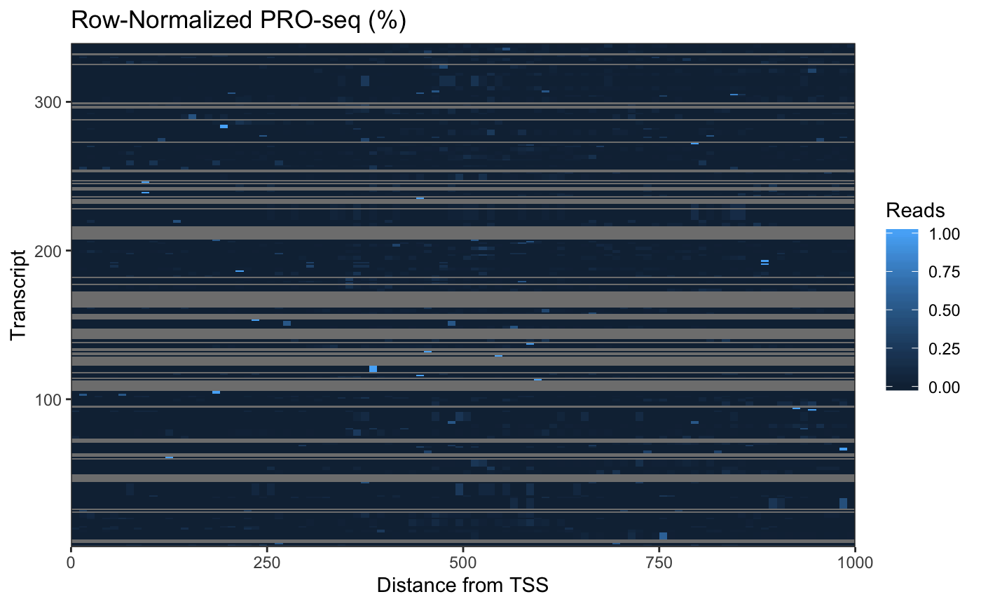

Efficient Analysis of Multiple Datasets

To efficiently work with several datasets, we recommend storing the GRanges objects within a standard, named list, e.g. grl <- list(a_rep1 = gr1, b_rep1 = gr2, ...).

library(BRGenomics)
data("PROseq")
data("txs_dm6_chr4")

# make 3 datasets
ps1 <- PROseq[seq(1, length(PROseq), 3)]
ps2 <- PROseq[seq(2, length(PROseq), 3)]
ps3 <- PROseq[seq(3, length(PROseq), 3)]

# use the "=" assignment in list() to give names to the list elements
ps_list <- list(ps1 = ps1, ps2 = ps2, ps3 = ps3)
names(ps_list)

## [1] "ps1" "ps2" "ps3"

ps_list

## $ps1
## GRanges object with 15794 ranges and 1 metadata column:
##           seqnames    ranges strand |     score
##              <Rle> <IRanges>  <Rle> | <integer>
##       [1]     chr4      1295      + |         1
##       [2]     chr4     42590      + |         2
##       [3]     chr4     42595      + |         1
##       [4]     chr4     42618      + |         1
##       [5]     chr4     42622      + |         2
##       ...      ...       ...    ... .       ...
##   [15790]     chr4   1307114      - |         1
##   [15791]     chr4   1307122      - |         1
##   [15792]     chr4   1307300      - |         1
##   [15793]     chr4   1316537      - |         1
##   [15794]     chr4   1319369      - |         1
##   -------
##   seqinfo: 7 sequences from an unspecified genome
## 
## $ps2
## GRanges object with 15793 ranges and 1 metadata column:
##           seqnames    ranges strand |     score
##              <Rle> <IRanges>  <Rle> | <integer>
##       [1]     chr4     41428      + |         1
##       [2]     chr4     42593      + |         5
##       [3]     chr4     42596      + |         1
##       [4]     chr4     42619      + |         2
##       [5]     chr4     42652      + |         3
##       ...      ...       ...    ... .       ...
##   [15789]     chr4   1307032      - |         1
##   [15790]     chr4   1307115      - |         2
##   [15791]     chr4   1307126      - |         1
##   [15792]     chr4   1307301      - |         1
##   [15793]     chr4   1318960      - |         1
##   -------
##   seqinfo: 7 sequences from an unspecified genome
## 
## $ps3
## GRanges object with 15793 ranges and 1 metadata column:
##           seqnames    ranges strand |     score
##              <Rle> <IRanges>  <Rle> | <integer>
##       [1]     chr4     42588      + |         1
##       [2]     chr4     42594      + |         2
##       [3]     chr4     42601      + |         1
##       [4]     chr4     42621      + |         1
##       [5]     chr4     42657      + |         1
##       ...      ...       ...    ... .       ...
##   [15789]     chr4   1307075      - |         1
##   [15790]     chr4   1307120      - |         1
##   [15791]     chr4   1307283      - |         1
##   [15792]     chr4   1307742      - |         1
##   [15793]     chr4   1319004      - |         1
##   -------
##   seqinfo: 7 sequences from an unspecified genome

A named list like the one above can be passed as an argument to nearly every function in BRGenomics, and many functions will automatically return dataframes, or melted dataframes that use the list names as the sample names (which can simplify plotting with ggplot2 or lattice).

Note that BRGenomics does also support the use of GRangesList or CompressedGRangesList classes for grouping multiple datasets. However, care should be taken when using these, as many functions with methods for GRanges objects also have methods for GRangesList objects. Furthermore, GRangesList objects can be automatically coerced into CompressedGRangesList objects, which can lower memory usage but can also incur significant performance penalties.

Example: Summarizing Signal from Multiple Samples

We can pass our list of GRanges directly to getCountsByRegions to simultaneously count reads for each dataset, and melt the result for plotting with ggplot:

getCountsByRegions(ps_list, txs_dm6_chr4[1:5], ncores = 1)

##   ps1 ps2 ps3
## 1   1   0   0
## 2  20  22  17
## 3   4   4   5
## 4  36  47  43
## 5  84  90  89

# melt, and use the optional region_names argument
txs_counts <- getCountsByRegions(ps_list, txs_dm6_chr4, melt = TRUE,
                                 region_names = txs_dm6_chr4$tx_name,
                                 ncores = 1)
head(txs_counts)

##        region signal sample
## 1 FBtr0346692      1    ps1
## 2 FBtr0344900     20    ps1
## 3 FBtr0340499      4    ps1
## 4 FBtr0333704     36    ps1
## 5 FBtr0333705     84    ps1
## 6 FBtr0100246   1017    ps1

library(ggplot2)
ggplot(txs_counts, aes(x = sample, y = signal, fill = sample)) + 
  geom_violin() + 
  theme_bw()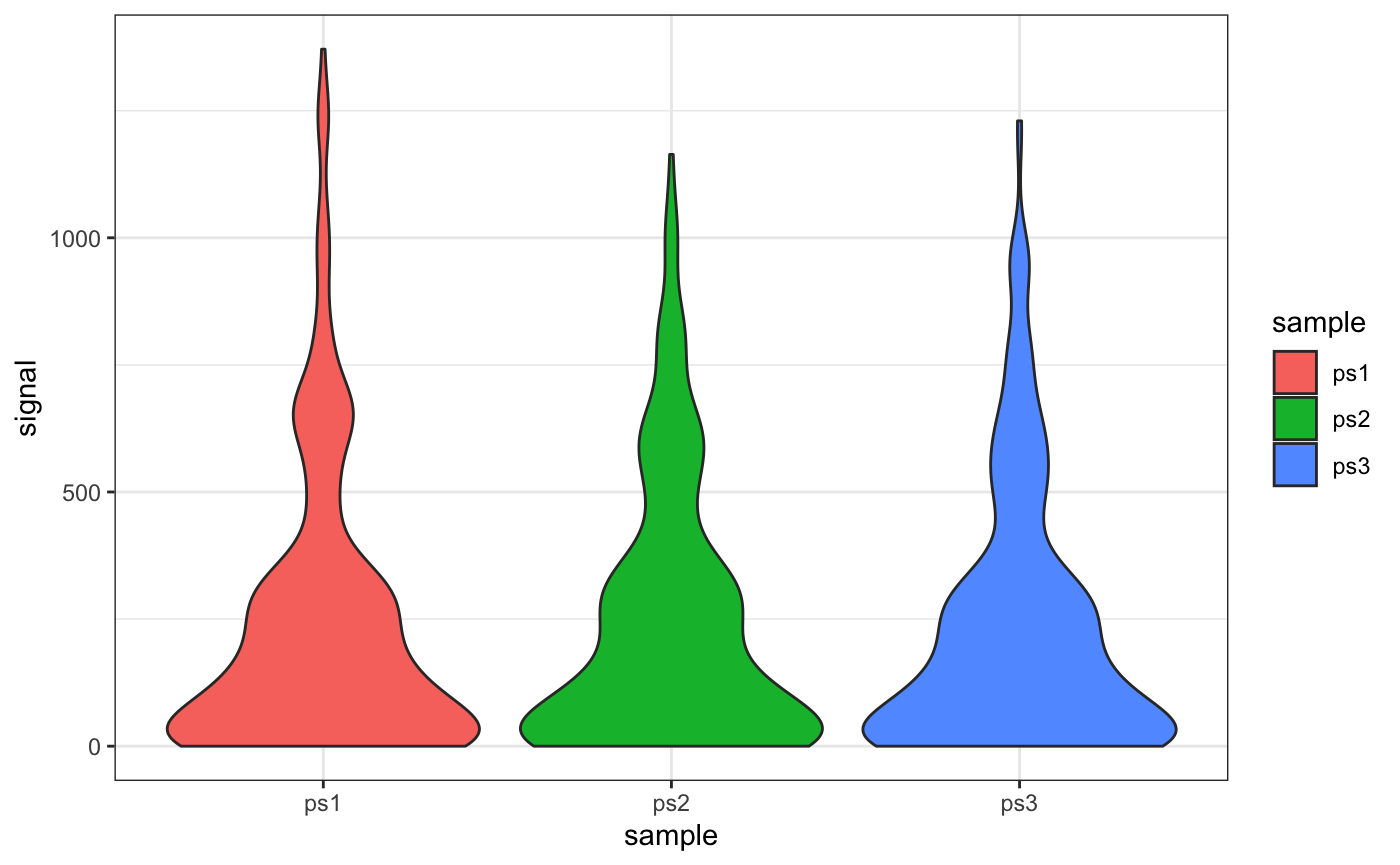

Example: Making Browser Shots in R

By using the getCountsByPositions on several datasets over a single region-of- interest, we can bake our own genome browser shots within R. Using the same region we plotted earlier:

cbp_maxtx <- getCountsByPositions(ps_list, txs_dm6_chr4[idx], 
                                  melt = TRUE, ncores = 1)
head(cbp_maxtx)

##   region position signal sample
## 1      1        1      0    ps1
## 2      1        2      0    ps1
## 3      1        3      0    ps1
## 4      1        4      0    ps1
## 5      1        5      0    ps1
## 6      1        6      0    ps1

ggplot(cbp_maxtx, aes(x = position, y = signal)) + 
  facet_wrap(~sample, ncol = 1, strip.position = "left") + 
  geom_col(size = 0.5, color = "darkgray") +
  labs(title = txs_dm6_chr4$tx_name[idx],
       x = "Distance from TSS", y = "PRO-seq Signal") + 
  theme_bw()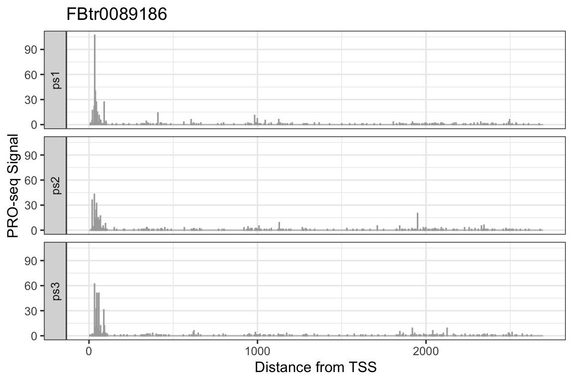

Multiplexed GRanges

There is another data structure that is widely supported with BRGenomics, called a multiplexed GRanges. A multiplexed GRanges is a single GRanges object that contains multiple metadata fields containing basepair-resolution coverage data for different datasets. We currently recommend users use lists of GRanges objects, but you might find that multiplexed GRanges objects have performance benefits for your data (notes on this below).

A multiplexed GRanges object can be made using the mergeGRangesData with option multiplex = TRUE.

ps_multi <- mergeGRangesData(ps1, ps2, ps3, multiplex = TRUE, ncores = 1)
ps_multi

## GRanges object with 47380 ranges and 3 metadata columns:
##           seqnames    ranges strand |       ps1       ps2       ps3
##              <Rle> <IRanges>  <Rle> | <integer> <integer> <integer>
##       [1]     chr4      1295      + |         1         0         0
##       [2]     chr4     41428      + |         0         1         0
##       [3]     chr4     42588      + |         0         0         1
##       [4]     chr4     42590      + |         2         0         0
##       [5]     chr4     42593      + |         0         5         0
##       ...      ...       ...    ... .       ...       ...       ...
##   [47376]     chr4   1307742      - |         0         0         1
##   [47377]     chr4   1316537      - |         1         0         0
##   [47378]     chr4   1318960      - |         0         1         0
##   [47379]     chr4   1319004      - |         0         0         1
##   [47380]     chr4   1319369      - |         1         0         0
##   -------
##   seqinfo: 7 sequences from an unspecified genome

As in any GRanges object, the metadata fields are accessible as a dataframe with the mcols() function, and individual columns are accessible with the $ operator.⁶

mcols(ps_multi)

## DataFrame with 47380 rows and 3 columns
##             ps1       ps2       ps3
##       <integer> <integer> <integer>
## 1             1         0         0
## 2             0         1         0
## 3             0         0         1
## 4             2         0         0
## 5             0         5         0
## ...         ...       ...       ...
## 47376         0         0         1
## 47377         1         0         0
## 47378         0         1         0
## 47379         0         0         1
## 47380         1         0         0

ps_multi$ps1[1:5]
## [1] 1 0 0 2 0

This data structure can be passed to most functions in BRGenomics. To be explicit, users should set the field argument, when it exists, to set the datasets for which calculations should be performed:

# for all datasets (all fields), get counts in the first 5 transcripts
getCountsByRegions(ps_multi, txs_dm6_chr4[1:5], 
                   field = names(mcols(ps_multi)),
                   ncores = 1)

##   ps1 ps2 ps3
## 1   1   0   0
## 2  20  22  17
## 3   4   4   5
## 4  36  47  43
## 5  84  90  89

# get counts for ps2 dataset only
getCountsByRegions(ps_multi, txs_dm6_chr4[1:5], 
                   field = "ps2", ncores = 1)

## [1]  0 22  4 47 90

# if no field is given, most functions will default to using all fields
getCountsByRegions(ps_multi, txs_dm6_chr4[1:5], 
                   ncores = 1)

## field not found in dataset.gr; will default to using all fields in dataset.gr

##   ps1 ps2 ps3
## 1   1   0   0
## 2  20  22  17
## 3   4   4   5
## 4  36  47  43
## 5  84  90  89

In our experience with PRO-seq data, and to our surprise, a list of GRanges objects typically outperforms multiplexed GRanges on a typical laptop, despite the theoretical benefits of multiplexing.

In principle, the multiplexed GRanges structure is designed to reduce memory usage and increase performance, but this has not been our experience when dealing with sparse, basepair-resolution data like PRO-seq. Overlapping signal with regions of interest (e.g. in getCountsByRegions or getCountsByPosition) is relatively efficient for reasonably sized GRanges objects, and these calculations scale reasonably well with multicore processing. While multiplexing means that signal overlapping only has to be performed once, we’ve found that this is a relatively small benefit in practice that is easily offset by having to do signal calculations on large sparse vectors of signal counts. However, the relative benefits of using lists or multiplexing are likely to depend on the nature of the data being analyzed, as well as well as computer hardware.

Saving Binary R Files

While the handling of GRanges data in BRGenomics is relatively fast, the initial importation of bigWig or bedGraph files as GRanges objects remains a noticeable bottleneck. This may be tolerable for interactive workflows, in which data is imported once before undergoing lengthy analysis, but the bottleneck is a significant detriment for users who regularly import data.

To avoid this bottleneck, users can save reusable data structures as binary R files, which effectively save the memory state of R objects. Not only are these objects rapidly reloaded into memory upon importation, but they have the added benefit of saving the user from repeating data formatting.

Any R object can be saved to storage using the saveRDS function, and re-imported using readRDS.

# save the PRO-seq GRanges for later import
saveRDS(PROseq, file = "~/PROseq.RData") 

# save a list of GRanges
saveRDS(ps_list, file = "~/ps_list.RData")

# re-import
ps_list <- readRDS("~/ps_list.RData")

The save and load commands can also be used to accomplish the same thing, although they work slightly differently.⁷

Profile Plots & Bootstrapping

Conventional Profiles

As an example, we’ll plot PRO-seq signal in promoter-proximal regions by calculating the mean signal intensity at each base in the first 100 bases of a transcript.

First, calculate signal at each base for all promoter-proximal regions:

library(BRGenomics)
data("PROseq")
data("txs_dm6_chr4")
txs_pr <- promoters(txs_dm6_chr4, 0, 100)

countmatrix_pr <- getCountsByPositions(PROseq, txs_pr, ncores = 1)
dim(countmatrix_pr)
## [1] 339 100
dim(countmatrix_pr) == c(length(txs_pr), unique(width(txs_pr)))
## [1] TRUE TRUE

For each position (each column of the matrix), calculate the mean, and plot:

plot(x = 1:ncol(countmatrix_pr),
     y = colMeans(countmatrix_pr),
     type = "l", 
     xlab = "Distance to TSS (bp)",
     ylab = "Mean PRO-seq Reads")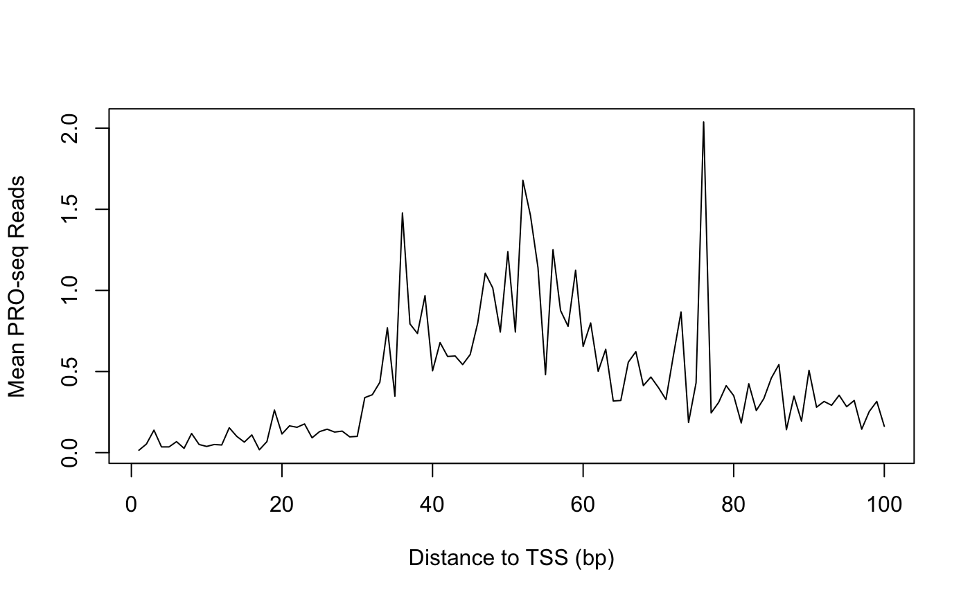

One drawback of using the arithmatic mean is that means are not robust to outliers. In other words, the mean signal at any position is liable to be determined by a small number of highly influential points. This is especially problematic for high dynamic range data like PRO-seq.

It’s common to see this issue addressed through the use medians/quantiles in place of arithmatic means. However, observe what happens as we plot the median signal across our gene list using several different gene-filtering thresholds:

plot_meds <- function(sig_thresh) {
  idx <- which(rowSums(countmatrix_pr) > sig_thresh)
  plot(x = 1:ncol(countmatrix_pr),
       y = apply(countmatrix_pr[idx, ], 2, median),
       type = "l", 
       main = sprintf("Regions with >%s reads", sig_thresh),
       xlab = "Distance to TSS (bp)",
       ylab = "Median PRO-seq Reads")
}

par(mfrow = c(3, 2))

for (i in c(0, 30*2^(0:4))) {
  plot_meds(i)
}

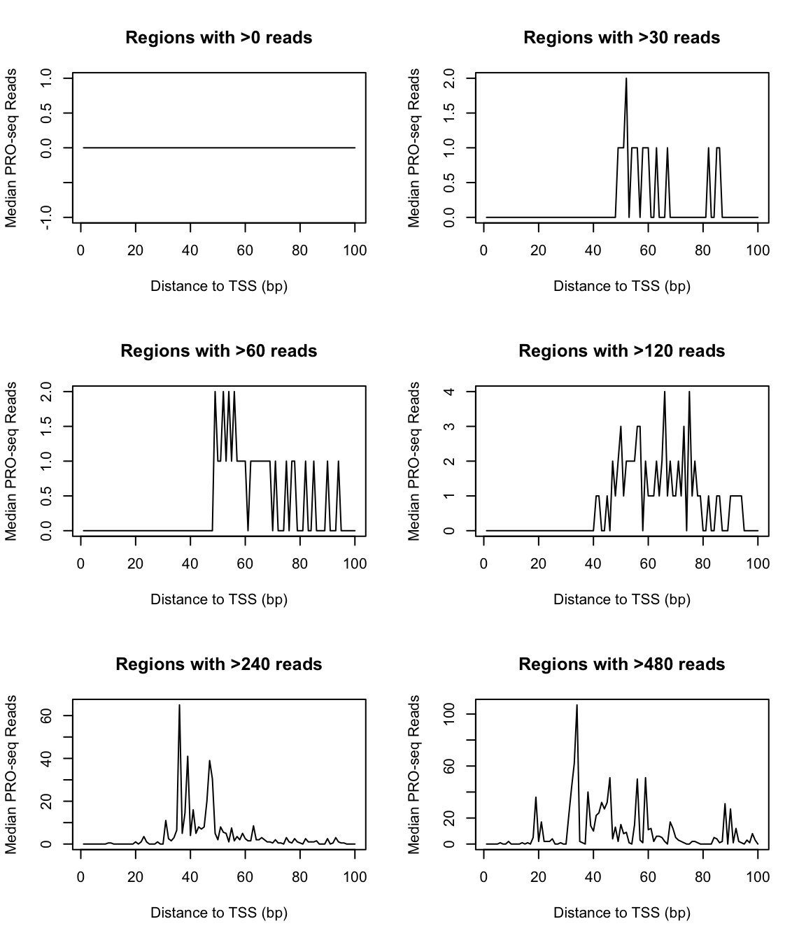
The paucity of transcription on Drosophila chromosome 4 makes this a somewhat extreme example, and you might find that the above situation is a non-issue for your data. However, it’s important to keep in mind how unexpressed genes can affect the median. A common rule of thumb is that a given cell is only apt to express around half of its genes; if that holds true, the median of an unfiltered genelist will be close to zero, and could be insensitive to changes occuring at expressed genes.

The Rationale for Bootstrapping

A robust alternative to plotting mean or median signal profiles is to plot bootstrapped mean signal profiles, known as metaprofile plots or metaplots.

To bootstrap the mean signal by position, a small number of genes are randomly sampled from a genelist, and the mean signal at each position is calculated for that group of genes. This process of randomly sampling genes and calculating mean signals is repeated over many iterations, and the final bootstrapped mean for each position is the median of the sampled means.

One feature of bootstrapping is that it is robust to outliers. But more than that, the a bootstrapped mean provides an expectation for what the mean signal would be for any arbitrary group of genes, and associated with that expectation is a measure of uncertainty. By taking quantiles of the subsampled means other than the median (the expected value), we can estimate the extent to which the mean varies across arbitrary groups of genes.

For example, the 75th percentile of the subsampled means is a number for which, 25% of the time, we calculated a higher mean. Similarly, a 90% confidence interval about the bootstrapped mean encompasses all values between the 5th and 95th percentiles of the subsampled means.

Generating and Plotting Metaprofiles

We can use the metaSubsample function to bootstrap mean values by position for a genelist. The function accepts the same arguments as getCountsByPositions, in addition to other arguments related to the bootstrapping.

By default, 10% of the genelist is randomly sampled 1000 times, and confidence bands are returned for the 12.5th and 87.5th percentiles (i.e. a 75% confidence interval).

Given the small size our dataset, we’ll reduce this to a 30% confidence interval, and we’ll additionally use 5 bp bins:

bootmeans.df <- metaSubsample(PROseq, txs_pr, binsize = 5, 
                              lower = 0.35, upper = 0.65, ncores = 1)
head(bootmeans.df)

##    x       mean      lower      upper sample.name
## 1  3 0.03529412 0.02941176 0.04705882      PROseq
## 2  8 0.05294118 0.04117647 0.07058824      PROseq
## 3 13 0.07647059 0.05294118 0.10000000      PROseq
## 4 18 0.07058824 0.05294118 0.09411765      PROseq
## 5 23 0.12941176 0.10000000 0.15882353      PROseq
## 6 28 0.09411765 0.08235294 0.10588235      PROseq

A dataframe is returned for plotting, and notice how the x-values have been automatically adjusted to be the center of the bins.

Below, we show how to plot the confidence bands using base R plotting, as well as ggplot2.

plot(mean ~ x, data = bootmeans.df, type = "l", 
     main = "PRO-seq Signal", ylim = c(0, 1.4),
     xlab = "Distance from TSS",
     ylab = "Mean Signal + 30% CI")

# draw a polygon to add confidence bands,
# and use adjustcolor() to add transparency
polygon(c(bootmeans.df$x, rev(bootmeans.df$x)), 
        c(bootmeans.df$lower, rev(bootmeans.df$upper)),
        col = adjustcolor("black", 0.1), border = FALSE)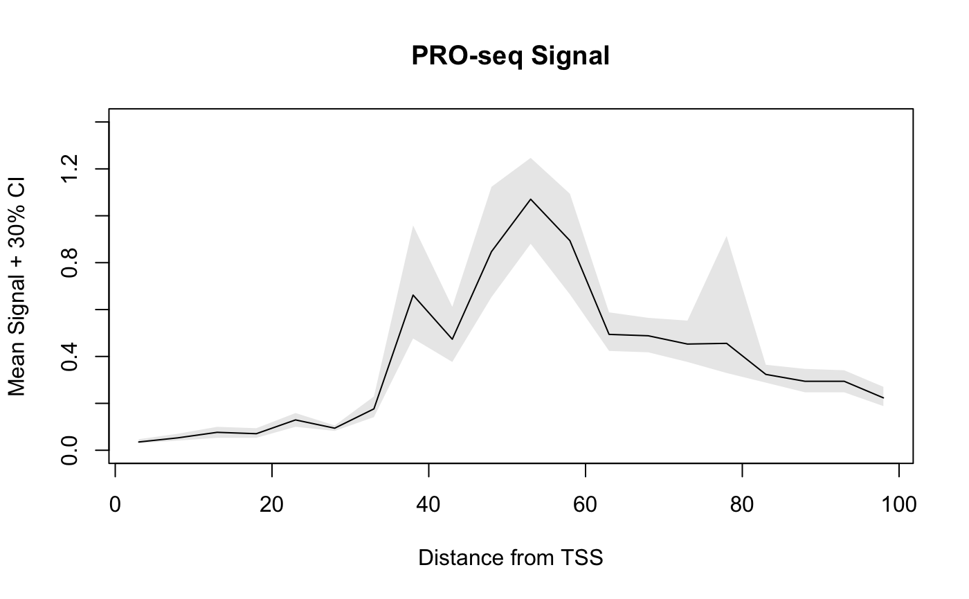

require(ggplot2)
ggplot(bootmeans.df, aes(x, mean)) + 
  geom_line() + 
  geom_ribbon(aes(x, ymin = lower, ymax = upper),
              alpha = 0.1) + 
  labs(title = "PRO-seq Signal", 
       x = "Distance from TSS", 
       y = "Mean Signal + 30% CI") + 
  theme_bw()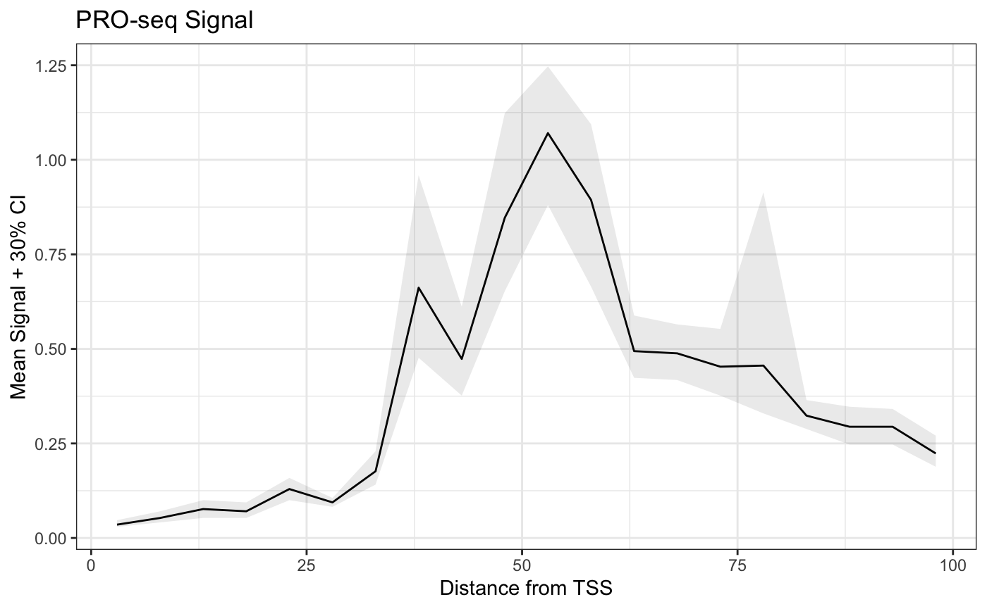

Example: Comparative Metaplots

Like other functions in BRGenomics, we can pass a list of GRanges to metaSubsample, and the output is conveniently combined for plotting.

bm_list.df <- metaSubsample(ps_list, txs_pr, binsize = 5, 
                            lower = 0.35, upper = 0.65, ncores = 1)
head(bm_list.df)

##    x       mean       lower      upper sample.name
## 1  3 0.01176471 0.005882353 0.01764706         ps1
## 2  8 0.01764706 0.011764706 0.02352941         ps1
## 3 13 0.01764706 0.011764706 0.02352941         ps1
## 4 18 0.04117647 0.023529412 0.05294118         ps1
## 5 23 0.02941176 0.021470588 0.04705882         ps1
## 6 28 0.02941176 0.023529412 0.04117647         ps1

require(ggplot2)
ggplot(bm_list.df, aes(x, mean, color = sample.name)) + 
  geom_line() + 
  geom_ribbon(aes(x, ymin = lower, ymax = upper,
                  color = NULL, fill = sample.name),
              alpha = 0.2) + 
  labs(title = "PRO-seq Signal", 
       x = "Distance from TSS", 
       y = "Mean Signal + 30% CI") + 
  theme_bw()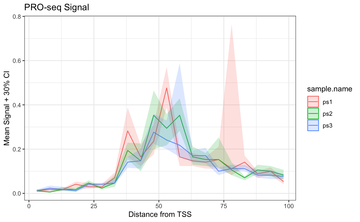

Bear in mind that the above confidence intervals are ignoring 70% of the subsampling experiments, which is excessive. More reasonable parameters would reveal how lacking this data is, i.e. how un-confident we are that there is a robust difference in the mean signal at various positions.

Spike-in Normalization

BRGenomics includes useful utilities for spike-in normalization.

A typical approach is to add the spike-in (either exogenous cells or synthetic oligonucleotides) before library preparation, and to subsequently map to a combined genome containing both the target organisms chromosomes (to map the experimental reads) as well as sequences/chromosomes for the spike-in.

This so-called “competitive alignment” results in the creation of BAM files containing a mix of chromosomes, for which it should be straightforward to identify the spike-in chromosomes.

Counting Spike-in Reads

library(BRGenomics)

For this section, we’ll use a list of 4 dummy datasets containing normal, as well as spike-in chromosomes. Consider the first 2 datasets:

grl[1:2]

## $gr1_rep1
## GRanges object with 4 ranges and 1 metadata column:
##        seqnames    ranges strand |     score
##           <Rle> <IRanges>  <Rle> | <numeric>
##   [1]      chr1         1      + |         1
##   [2]      chr2         2      + |         1
##   [3] spikechr1         3      + |         1
##   [4] spikechr2         4      + |         1
##   -------
##   seqinfo: 4 sequences from an unspecified genome; no seqlengths
## 
## $gr2_rep1
## GRanges object with 4 ranges and 1 metadata column:
##        seqnames    ranges strand |     score
##           <Rle> <IRanges>  <Rle> | <numeric>
##   [1]      chr1         1      + |         2
##   [2]      chr2         2      + |         2
##   [3] spikechr1         3      + |         1
##   [4] spikechr2         4      + |         1
##   -------
##   seqinfo: 4 sequences from an unspecified genome; no seqlengths

We can identify the spike-in chromosomes either by full names, or by a regular expression that matches the spike-in chromosomes. In this case, we named our spike-in chromosomes to contain the string “spike” which makes them easy to identify.

To count the reads for each dataset:

getSpikeInCounts(grl, si_pattern = "spike", ncores = 1)

##     sample total_reads exp_reads spike_reads
## 1 gr1_rep1           4         2           2
## 2 gr2_rep1           6         4           2
## 3 gr1_rep2           5         2           3
## 4 gr2_rep2          12         8           4

Filtering Spike-in Reads

We can also remove the spike-in reads from our data:

removeSpikeInReads(grl[1:2], si_pattern = "spike", ncores = 1)

## $gr1_rep1
## GRanges object with 2 ranges and 1 metadata column:
##       seqnames    ranges strand |     score
##          <Rle> <IRanges>  <Rle> | <numeric>
##   [1]     chr1         1      + |         1
##   [2]     chr2         2      + |         1
##   -------
##   seqinfo: 2 sequences from an unspecified genome; no seqlengths
## 
## $gr2_rep1
## GRanges object with 2 ranges and 1 metadata column:
##       seqnames    ranges strand |     score
##          <Rle> <IRanges>  <Rle> | <numeric>
##   [1]     chr1         1      + |         2
##   [2]     chr2         2      + |         2
##   -------
##   seqinfo: 2 sequences from an unspecified genome; no seqlengths

And if we wanted to isolate the spike-in reads, there is an analagous getSpikeInReads() function.

The Spike-in Normalization Factor

There are several methods by which to generate spike-in normalization factors, but we advocate for a particular method, which generates units we call Spike-in normalized Reads Per Million mapped reads in the negative Control (SRPMC). The SRPMC normalization factor for a given sample $i$ is defined as such:

\[SRPMC:\ NF_i = \frac{\sum reads_{spikein, control}}{\sum reads_{spikein, i}} \cdot \frac{10^6}{\sum reads_{experimental, control}}\]

This expression effectively calculates Reads Per Million (RPM) normalization for the negative control, and all other samples $i$ are scaled into equivalent units according to the ratio of their spike-in reads. We provide a more explicit derivation below.

Derivation of SRPMC

The fundamental concept of spike-in normalization is that the ratio of experimental reads to spike-in reads can be used to correct for global changes in starting material. Let’s call this ratio Reads Per Spike-in read (RPS):

\[RPS = \frac{\sum reads_{experimental}}{\sum reads_{spikein}}\]

In isolation, this number only reflects the relative amounts of spike-in material recovered and mapped. The meaningful information about changes in material can only arise from making direct comparisons between samples. For any sample, $i$, we can calculate the global change in signal as a proportion of the material recovered from a negative control:

\[RelativeSignal_i = \frac{RPS_i}{RPS_{control}}\]

The usual purpose of spike-in normalization is to measure a biological difference in total material (e.g. RNA) between samples, and the above ratio is a direct measurement of this.

To generate normalization factors, we use the above ratio to adjust RPM (Reads Per Million mapped reads) normalization factors, which we define below for clarity:

\[RPM:\ NF_i = \frac{1}{\frac{\sum{reads_i}}{10^6}} = \frac{10^6}{\sum{reads_i}}\]

(Unless indicated, $reads$ refers to non-spike-in reads).

RPM normalization (i.e. read depth normalization) is the simplest and likely most familiar form of normalization. For a basal (unperturbed) negative control, RPM should produce the most portable metric of signal, given that we intend for the negative control to demonstrate typical physiology, and we hope that this state is reproducible. We therefore want to have our normalized signal in unit terms of RPM in the negative control.

To accomplish this, we multiply the ratio of spike-in normalized reads between the sample $i$ and the negative control to the RPM normalization factor for sample $i$. This converts readcounts into units we summarize as Spike-in normalized Reads Per Million mapped reads in the negative Control (SRPMC):

\[SRPMC:\ NF_i = \frac{RPS_i}{RPS_{control}} \cdot \frac{10^6}{\sum{reads_i}}\]

Again, SRPMC results in the negative control being RPM (sequencing depth) normalized, while all other samples are in equivalent, directly comparable units. And we’ve effectively determined the relative scaling of those samples based on the ratios of spike-in reads.

This becomes more apparent if we substitute the $RPS$ variables above. $\sum{reads_i}$ cancels, and simplifying the fraction produces the original formula:

\[SRPMC:\ NF_i = \frac{\sum reads_{spikein, control}}{\sum reads_{spikein, i}} \cdot \frac{10^6}{\sum reads_{experimental, control}}\]

Calculating Normalization Factors

We can calculate SRPMC normalization factors for each sample using the getSpikeInNFs() function, using the same syntax we used to count the spike-in reads.

However, we have to also identify the negative control, which is the sample that will have the “reference” (RPM) normalization. We do this either using a regular expression (ctrl_pattern argument) or by supplying the name(s) of the negative controls (the ctrl_names argument).

The default method is “SRPMC”, but there are other options, as well.

getSpikeInNFs(grl, si_pattern = "spike", ctrl_pattern = "gr1", ncores = 1)

## [1] 500000 500000 500000 375000

(The NFs are high because our dummy data contain only a few reads).

By default, normalization factors utilize batch normalization, such that in any replicate (identified by the characters following “rep” in the sample names), the negative control is RPM normalized, and the other conditions are normlized to the within-replicate negative control (see the documentation for further details).

Currently, batch normalization requires the sample names end with strings matching the format "_rep1", "_rep2", etc. If sample names do not conform to this pattern, you can rename them by using the sample_names argument.

Normalizing Data

We can also use the spikeInNormGRanges() function to simultaneously find the spike-in reads, calculate the spike-in normalization factors, filter out spike-in reads, and normalize the readcounts:

spikeInNormGRanges(grl, si_pattern = "spike", ctrl_pattern = "gr1", ncores = 1)

## $gr1_rep1
## GRanges object with 2 ranges and 1 metadata column:
##       seqnames    ranges strand |     score
##          <Rle> <IRanges>  <Rle> | <numeric>
##   [1]     chr1         1      + |     5e+05
##   [2]     chr2         2      + |     5e+05
##   -------
##   seqinfo: 2 sequences from an unspecified genome; no seqlengths
## 
## $gr2_rep1
## GRanges object with 2 ranges and 1 metadata column:
##       seqnames    ranges strand |     score
##          <Rle> <IRanges>  <Rle> | <numeric>
##   [1]     chr1         1      + |     1e+06
##   [2]     chr2         2      + |     1e+06
##   -------
##   seqinfo: 2 sequences from an unspecified genome; no seqlengths
## 
## $gr1_rep2
## GRanges object with 2 ranges and 1 metadata column:
##       seqnames    ranges strand |     score
##          <Rle> <IRanges>  <Rle> | <numeric>
##   [1]     chr1         1      + |     5e+05
##   [2]     chr2         2      + |     5e+05
##   -------
##   seqinfo: 2 sequences from an unspecified genome; no seqlengths
## 
## $gr2_rep2
## GRanges object with 2 ranges and 1 metadata column:
##       seqnames    ranges strand |     score
##          <Rle> <IRanges>  <Rle> | <numeric>
##   [1]     chr1         1      + |   1500000
##   [2]     chr2         2      + |   1500000
##   -------
##   seqinfo: 2 sequences from an unspecified genome; no seqlengths

Normalization by Subsampling

Rationale

When viewing genomics data in a genome browser (or otherwise plotting signal for a single gene), the sparsity of basepair resolution data can challenge our visual perception.

Consider two datasets from identical samples, but where one is sequenced to a higher depth. The two datasets can be normalized such that the signal counts are equivalent, but the dataset with higher sequencing depth will have also uncovered additional sites. When plotted in a genome browser, the total signal within a region may be the same, but the more highly sequenced dataset will cover more positions but have lower peaks, while the less sequenced dataset will look sparse and spikey in comparison.

Below, we compare PRO-seq data derived from the same dataset over the same gene. In one case, we randomly sample half of the reads over that gene, while in another, we divide all the readcounts by 2.

# choose a single gene
gene_i <- txs_dm6_chr4[185]
reads.gene_i <- subsetByOverlaps(PROseq, gene_i)

# sample half the raw reads
set.seed(11)
sreads.gene_i <- subsampleGRanges(reads.gene_i, prop = 0.5, ncores = 1)

# downscale raw reads by a factor of 2
score(reads.gene_i) <- 0.5 * score(reads.gene_i)

sum(score(reads.gene_i))
## [1] 738.5
sum(score(sreads.gene_i))
## [1] 738

plot(x = 1:width(gene_i), 
     y = getCountsByPositions(sreads.gene_i, gene_i),
     type = "h", ylim = c(0, 20),
     main = "PRO-seq (downsampled)",
     xlab = "Distance from TSS", ylab = "Downsampled PRO-seq Reads")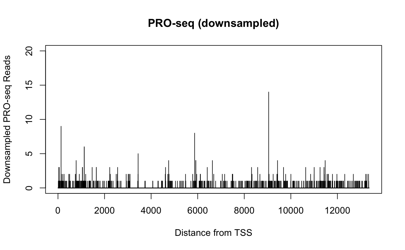

plot(x = 1:width(gene_i), 
     y = getCountsByPositions(reads.gene_i, gene_i),
     type = "h",  ylim = c(0, 20),
     main = "PRO-seq (downscaled)", 
     xlab = "Distance from TSS",  ylab = "Downscaled PRO-seq Reads")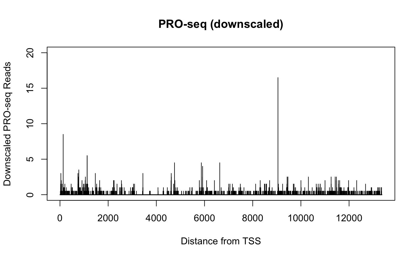

The two plots above come from the same data, and contain the same quantity of signal, but their profiles are notably distinct. Particularly when plotting many samples over large regions within a genome browser, differences caused by sequencing depth can be misleading. It can be challenging to estimate differences if some datasets are “tall and spikey” while others are “short and smooth”.

Absent global changes in signal, the above scenario can be resolved beforehand by equal sequencing depths, or by down-sampling to match readcounts.

However, matching raw readcounts is not a solution when significant biological changes in total signal should be accounted for.

For instance, consider an example in which there is a true, two-fold biological difference in transcription between two samples. If we could avoid all technical artifacts and measure the transcription directly in each individual cell, we would expect to uncover half the number of transcribing complexes in the lower condition. Having equivalent sequencing depth across those two conditions is effectively a technical artifact, and down-scaling the signal by multiplication can cause the visual challenges observed above.

Subsampling for Normalization

To address the above concerns, we’ve included a function subsampleBySpikeIn() to randomly sample reads to match the normalized signal proportions between datasets.

Internally, the function uses the getSpikeInNFs() function, but instead of SRPMC normalization, using the option method = "SNR", which calculates normalization factors that downscale each dataset to match the dataset with the least spike-in reads. From this, the number of “desired reads” is established for each dataset, and subsequently that number of reads is randomly sampled.

removeSpikeInReads(grl, si_pattern = "spike", ncores = 1)

## $gr1_rep1
## GRanges object with 2 ranges and 1 metadata column:
##       seqnames    ranges strand |     score
##          <Rle> <IRanges>  <Rle> | <numeric>
##   [1]     chr1         1      + |         1
##   [2]     chr2         2      + |         1
##   -------
##   seqinfo: 2 sequences from an unspecified genome; no seqlengths
## 
## $gr2_rep1
## GRanges object with 2 ranges and 1 metadata column:
##       seqnames    ranges strand |     score
##          <Rle> <IRanges>  <Rle> | <numeric>
##   [1]     chr1         1      + |         2
##   [2]     chr2         2      + |         2
##   -------
##   seqinfo: 2 sequences from an unspecified genome; no seqlengths
## 
## $gr1_rep2
## GRanges object with 2 ranges and 1 metadata column:
##       seqnames    ranges strand |     score
##          <Rle> <IRanges>  <Rle> | <numeric>
##   [1]     chr1         1      + |         1
##   [2]     chr2         2      + |         1
##   -------
##   seqinfo: 2 sequences from an unspecified genome; no seqlengths
## 
## $gr2_rep2
## GRanges object with 2 ranges and 1 metadata column:
##       seqnames    ranges strand |     score
##          <Rle> <IRanges>  <Rle> | <numeric>
##   [1]     chr1         1      + |         4
##   [2]     chr2         2      + |         4
##   -------
##   seqinfo: 2 sequences from an unspecified genome; no seqlengths

getSpikeInNFs(grl, si_pattern = "spike", method = "SNR", batch_norm = FALSE,
              ncores = 1)

## [1] 1.0000000 1.0000000 0.6666667 0.5000000

subsampleBySpikeIn(grl, si_pattern = "spike", batch_norm = FALSE, ncores = 1)

## $gr1_rep1
## GRanges object with 2 ranges and 1 metadata column:
##       seqnames    ranges strand |     score
##          <Rle> <IRanges>  <Rle> | <integer>
##   [1]     chr1         1      + |         1
##   [2]     chr2         2      + |         1
##   -------
##   seqinfo: 2 sequences from an unspecified genome; no seqlengths
## 
## $gr2_rep1
## GRanges object with 2 ranges and 1 metadata column:
##       seqnames    ranges strand |     score
##          <Rle> <IRanges>  <Rle> | <integer>
##   [1]     chr1         1      + |         2
##   [2]     chr2         2      + |         2
##   -------
##   seqinfo: 2 sequences from an unspecified genome; no seqlengths
## 
## $gr1_rep2
## GRanges object with 1 range and 1 metadata column:
##       seqnames    ranges strand |     score
##          <Rle> <IRanges>  <Rle> | <integer>
##   [1]     chr1         1      + |         1
##   -------
##   seqinfo: 2 sequences from an unspecified genome; no seqlengths
## 
## $gr2_rep2
## GRanges object with 2 ranges and 1 metadata column:
##       seqnames    ranges strand |     score
##          <Rle> <IRanges>  <Rle> | <integer>
##   [1]     chr1         1      + |         1
##   [2]     chr2         2      + |         3
##   -------
##   seqinfo: 2 sequences from an unspecified genome; no seqlengths

Normalization by subsampling sacrifices information to reduce biases across datasets.

Using DESeq2 for Pairwise Differential Expression

Rationale

DESeq2’s default treatment of data relies on the assumption that genewise estimates of dispersion are largely unchanged across samples. While this assumption holds for a typical RNA-seq data, it can be violated if there are samples within the DESeqDataSet object for which there are meaningful signal changes across a majority of regions of interest.

The BRGenomics functions getDESeqDataSet() and getDESeqResults() are simple and flexible wrappers for making pairwise comparisons between individual samples, without relying on the assumption of globally-similar dispersion estimates. In particular, getDESeqResults() follows the logic that the presence of a dataset $X$ within the DESeqDataSet object will not affect the comparison of datasets $Y$ and $Z$.

While the intuition above is appealing, users should note that if the globally-similar dispersions assumption does hold, then DESeq2’s default behavior should be more sensitive in its estimates of genewise dispersion. In this case, users can still take advantage of the convenience of the BRGenomics function getDESeqDataSet(), but they should subsequently call DESeq2::DESeq() and DESeq2::results() directly.

If the globally-similar dispersions assumption is violated, but something beyond simple pairwise comparisons is desired (e.g. group comparisons or additional model terms), we note that, with some prying, DESeq2 can be used without “blind dispersion estimation” (see the DESeq2 manual).

Formatting Data for DESeq2

Just like the functions that generate batch-normalized spike-in normalization factors, the DESeq-oriented functions require that the names of the input datasets end in "rep1", "rep2", etc.

We’ll use another list of GRanges here, in order to have multiple comparisons to make:

ps_list2 <- lapply(1:6, function(i) PROseq[seq(i, length(PROseq), 6)])
names(ps_list2) <- c("A_rep1", "A_rep2", 
                     "B_rep1", "B_rep2",
                     "C_rep1", "C_rep2")

ps_list2[1:2]

## $A_rep1
## GRanges object with 7897 ranges and 1 metadata column:
##          seqnames    ranges strand |     score
##             <Rle> <IRanges>  <Rle> | <integer>
##      [1]     chr4      1295      + |         1
##      [2]     chr4     42595      + |         1
##      [3]     chr4     42622      + |         2
##      [4]     chr4     42718      + |         1
##      [5]     chr4     42789      + |         1
##      ...      ...       ...    ... .       ...
##   [7893]     chr4   1295277      - |         1
##   [7894]     chr4   1306500      - |         1
##   [7895]     chr4   1306889      - |         1
##   [7896]     chr4   1307122      - |         1
##   [7897]     chr4   1316537      - |         1
##   -------
##   seqinfo: 7 sequences from an unspecified genome
## 
## $A_rep2
## GRanges object with 7897 ranges and 1 metadata column:
##          seqnames    ranges strand |     score
##             <Rle> <IRanges>  <Rle> | <integer>
##      [1]     chr4     41428      + |         1
##      [2]     chr4     42596      + |         1
##      [3]     chr4     42652      + |         3
##      [4]     chr4     42733      + |         1
##      [5]     chr4     42794      + |         2
##      ...      ...       ...    ... .       ...
##   [7893]     chr4   1305972      - |         1
##   [7894]     chr4   1306514      - |         1
##   [7895]     chr4   1307032      - |         1
##   [7896]     chr4   1307126      - |         1
##   [7897]     chr4   1318960      - |         1
##   -------
##   seqinfo: 7 sequences from an unspecified genome

names(ps_list2)

## [1] "A_rep1" "A_rep2" "B_rep1" "B_rep2" "C_rep1" "C_rep2"

As you can see, the names all end in “repX”, where X indicates the replicate. Replicates will be grouped by anything that follows “rep”. If the sample names do not conform to this standard, the sample_names argument can be used to rename the samples within the call to getDESeqDataSet().

dds <- getDESeqDataSet(ps_list2, txs_dm6_chr4,
                       gene_names = txs_dm6_chr4$gene_id,
                       ncores = 1)
dds

## class: DESeqDataSet 
## dim: 111 6 
## metadata(1): version
## assays(1): counts
## rownames(111): FBgn0267363 FBgn0266617 ... FBgn0039924 FBgn0027101
## rowData names(2): tx_name gene_id
## colnames(6): A_rep1 A_rep2 ... C_rep1 C_rep2
## colData names(2): condition replicate

Notice that the dim attribute of the DESeqDataSet object is c(111, 6). There are 6 samples, but length(txs_dm6_chr4) is not 111. This is because we provided gene names to getDESeqDataSet(), which were non-unique. The feature being exploited here is for use with discontinuous gene regions, not for multiple overlapping transcript isoforms.

By default, getDESeqDataSet() will combine counts across all ranges belonging to a gene, but if they overlap, they will be counted twice. For addressing issues related to overlaps, see the reduceByGene() and intersectByGene() functions.

We could have added normalization factors, which DESeq2 calls “size factors”, in the call to getDESeqDataSet(), or we can supply them to getDESeqResults() below. (Supplying them twice will overwrite the previous size factors).

Important note on normalization factors: DESeq2 “size factors” are the inverse of BRGenomics normalization factors. So if you calculate normalization factors with NF <- getSpikeInNFs(...), set sizeFactors <- 1/NF.

Getting DESeq2 Results

Generating DESeq2 results is simple:

getDESeqResults(dds, contrast.numer = "B", contrast.denom = "A",
                quiet = TRUE, ncores = 1)

## log2 fold change (MLE): condition B vs A 
## Wald test p-value: condition B vs A 
## DataFrame with 111 rows and 6 columns
##                baseMean log2FoldChange     lfcSE       stat    pvalue      padj
##               <numeric>      <numeric> <numeric>  <numeric> <numeric> <numeric>
## FBgn0267363    0.252443     -1.4201507  4.997269 -0.2841853  0.776268  0.990374
## FBgn0266617    9.648855     -0.4357749  0.983164 -0.4432374  0.657594  0.990374
## FBgn0265633    2.291440      0.3467829  1.882149  0.1842484  0.853819  0.990374
## FBgn0264617   67.131764      0.0245325  0.451334  0.0543556  0.956652  0.990374
## FBgn0085432 4688.232636     -0.0469812  0.270431 -0.1737268  0.862080  0.990374
## ...                 ...            ...       ...        ...       ...       ...
## FBgn0039928     653.783    -0.00994936  0.262637 -0.0378825  0.969781  0.990374
## FBgn0052017     114.906     0.02350299  0.369082  0.0636796  0.949225  0.990374
## FBgn0002521     168.778     0.05777885  0.347249  0.1663903  0.867850  0.990374
## FBgn0039924     170.213    -0.20850730  0.409865 -0.5087219  0.610947  0.990374
## FBgn0027101     343.009    -0.21151750  0.290061 -0.7292177  0.465868  0.990374

We can also make multiple pairwise-comparisons by ignoring the contrast.numer and contrast.denom arguments, and instead using the comparisons argument. The resulting list of results is named according to the comparisons:

comparison_list <- list(c("B", "A"), 
                        c("C", "A"),
                        c("C", "B"))
dsres <- getDESeqResults(dds, comparisons = comparison_list,
                         quiet = TRUE, ncores = 1)
names(dsres)

## [1] "B_vs_A" "C_vs_A" "C_vs_B"

dsres$C_vs_B

## log2 fold change (MLE): condition C vs B 
## Wald test p-value: condition C vs B 
## DataFrame with 111 rows and 6 columns
##               baseMean log2FoldChange     lfcSE       stat    pvalue      padj
##              <numeric>      <numeric> <numeric>  <numeric> <numeric> <numeric>
## FBgn0267363    0.00000             NA        NA         NA        NA        NA
## FBgn0266617    9.38822      0.3938871  0.901764   0.436796  0.662259  0.998692
## FBgn0265633    2.28968     -0.3206785  1.718554  -0.186598  0.851976  0.998692
## FBgn0264617   65.30695     -0.0773192  0.415908  -0.185905  0.852520  0.998692
## FBgn0085432 4281.29059     -0.1902162  0.229704  -0.828094  0.407617  0.998692
## ...                ...            ...       ...        ...       ...       ...
## FBgn0039928    696.482      0.2150507  0.248408  0.8657159  0.386646  0.998692
## FBgn0052017    133.743      0.4160583  0.333948  1.2458762  0.212810  0.998692
## FBgn0002521    171.141      0.0159143  0.323995  0.0491188  0.960825  0.998692
## FBgn0039924    138.749     -0.3685073  0.327200 -1.1262461  0.260061  0.998692
## FBgn0027101    347.104      0.2699312  0.271542  0.9940675  0.320190  0.998692

Blacklisting

Many functions in BRGenomics support blacklisting, or the exclusion of certain sites from analysis. To use this feature, import your blacklist as a GRanges object, and use the blacklist option.

For instance, getCountsByPositions() supports blacklisting, and there is an additional option of whether to set all blacklisted sites to 0 counts, or to set those sites equal to NA. Setting them to NA is useful, as many functions have arguments to ignore NA values in calculations, i.e. mean(x, na.rm = TRUE).

Supplying a blacklist to metaSubsample() will result in blacklisted positions being ignored in the calculations. Regions for which some section overlaps the blacklist are not ignored entirely, but the blacklisted positions themselves won’t contribute to the calculations.

Merging GRanges Data

Biological replicates are best used to independently reproduce and measure effects, and therefore we often want to handle them separately. However, there are times when combining replicates can allow for more sensitive measurements, assuming that the replicates are highly concordant.

The mergeGRangesData() function can be used to combine basepair-resolution GRanges objects.

library(BRGenomics)
data("PROseq")

# make a number of GRanges
ps_list <- lapply(1:6, function(i) PROseq[seq(i, length(PROseq), 6)])
names(ps_list) <- c("A_rep1", "A_rep2", 
                    "B_rep1", "B_rep2",
                    "C_rep1", "C_rep2")

ps_list[1:2]

## $A_rep1
## GRanges object with 7897 ranges and 1 metadata column:
##          seqnames    ranges strand |     score
##             <Rle> <IRanges>  <Rle> | <integer>
##      [1]     chr4      1295      + |         1
##      [2]     chr4     42595      + |         1
##      [3]     chr4     42622      + |         2
##      [4]     chr4     42718      + |         1
##      [5]     chr4     42789      + |         1
##      ...      ...       ...    ... .       ...
##   [7893]     chr4   1295277      - |         1
##   [7894]     chr4   1306500      - |         1
##   [7895]     chr4   1306889      - |         1
##   [7896]     chr4   1307122      - |         1
##   [7897]     chr4   1316537      - |         1
##   -------
##   seqinfo: 7 sequences from an unspecified genome
## 
## $A_rep2
## GRanges object with 7897 ranges and 1 metadata column:
##          seqnames    ranges strand |     score
##             <Rle> <IRanges>  <Rle> | <integer>
##      [1]     chr4     41428      + |         1
##      [2]     chr4     42596      + |         1
##      [3]     chr4     42652      + |         3
##      [4]     chr4     42733      + |         1
##      [5]     chr4     42794      + |         2
##      ...      ...       ...    ... .       ...
##   [7893]     chr4   1305972      - |         1
##   [7894]     chr4   1306514      - |         1
##   [7895]     chr4   1307032      - |         1
##   [7896]     chr4   1307126      - |         1
##   [7897]     chr4   1318960      - |         1
##   -------
##   seqinfo: 7 sequences from an unspecified genome

names(ps_list)

## [1] "A_rep1" "A_rep2" "B_rep1" "B_rep2" "C_rep1" "C_rep2"

length(ps1)
## [1] 15794
length(ps2)
## [1] 15793
length(ps3)
## [1] 15793

We can pass any number of individual GRanges objects as arguments:

merge_ps <- mergeGRangesData(ps_list[[1]], ps_list[[2]], PROseq, ncores = 1)
merge_ps

## GRanges object with 47380 ranges and 1 metadata column:
##           seqnames    ranges strand |     score
##              <Rle> <IRanges>  <Rle> | <integer>
##       [1]     chr4      1295      + |         2
##       [2]     chr4     41428      + |         2
##       [3]     chr4     42588      + |         1
##       [4]     chr4     42590      + |         2
##       [5]     chr4     42593      + |         5
##       ...      ...       ...    ... .       ...
##   [47376]     chr4   1307742      - |         1
##   [47377]     chr4   1316537      - |         2
##   [47378]     chr4   1318960      - |         2
##   [47379]     chr4   1319004      - |         1
##   [47380]     chr4   1319369      - |         1
##   -------
##   seqinfo: 7 sequences from an unspecified genome

Note that the output is also a basepair-resolution GRanges object:

isBRG(merge_ps)
## [1] TRUE

Or we could also pass a list of GRanges objects directly as an argument:

mergeGRangesData(ps_list, ncores = 1)

## GRanges object with 47380 ranges and 1 metadata column:
##           seqnames    ranges strand |     score
##              <Rle> <IRanges>  <Rle> | <integer>
##       [1]     chr4      1295      + |         1
##       [2]     chr4     41428      + |         1
##       [3]     chr4     42588      + |         1
##       [4]     chr4     42590      + |         2
##       [5]     chr4     42593      + |         5
##       ...      ...       ...    ... .       ...
##   [47376]     chr4   1307742      - |         1
##   [47377]     chr4   1316537      - |         1
##   [47378]     chr4   1318960      - |         1
##   [47379]     chr4   1319004      - |         1
##   [47380]     chr4   1319369      - |         1
##   -------
##   seqinfo: 7 sequences from an unspecified genome

The mergeReplicates() function makes combining replicates particularly simple:

mergeReplicates(ps_list, ncores = 1)

## $A
## GRanges object with 15794 ranges and 1 metadata column:
##           seqnames    ranges strand |     score
##              <Rle> <IRanges>  <Rle> | <integer>
##       [1]     chr4      1295      + |         1
##       [2]     chr4     41428      + |         1
##       [3]     chr4     42595      + |         1
##       [4]     chr4     42596      + |         1
##       [5]     chr4     42622      + |         2
##       ...      ...       ...    ... .       ...
##   [15790]     chr4   1307032      - |         1
##   [15791]     chr4   1307122      - |         1
##   [15792]     chr4   1307126      - |         1
##   [15793]     chr4   1316537      - |         1
##   [15794]     chr4   1318960      - |         1
##   -------
##   seqinfo: 7 sequences from an unspecified genome
## 
## $B
## GRanges object with 15794 ranges and 1 metadata column:
##           seqnames    ranges strand |     score
##              <Rle> <IRanges>  <Rle> | <integer>
##       [1]     chr4     42588      + |         1
##       [2]     chr4     42590      + |         2
##       [3]     chr4     42601      + |         1
##       [4]     chr4     42618      + |         1
##       [5]     chr4     42657      + |         1
##       ...      ...       ...    ... .       ...
##   [15790]     chr4   1307114      - |         1
##   [15791]     chr4   1307283      - |         1
##   [15792]     chr4   1307300      - |         1
##   [15793]     chr4   1319004      - |         1
##   [15794]     chr4   1319369      - |         1
##   -------
##   seqinfo: 7 sequences from an unspecified genome
## 
## $C
## GRanges object with 15792 ranges and 1 metadata column:
##           seqnames    ranges strand |     score
##              <Rle> <IRanges>  <Rle> | <integer>
##       [1]     chr4     42593      + |         5
##       [2]     chr4     42594      + |         2
##       [3]     chr4     42619      + |         2
##       [4]     chr4     42621      + |         1
##       [5]     chr4     42661      + |         1
##       ...      ...       ...    ... .       ...
##   [15788]     chr4   1306888      - |         1
##   [15789]     chr4   1307115      - |         2
##   [15790]     chr4   1307120      - |         1
##   [15791]     chr4   1307301      - |         1
##   [15792]     chr4   1307742      - |         1
##   -------
##   seqinfo: 7 sequences from an unspecified genome

Sequence Extraction

In this section, we’ll give one more example showing the benefit of Bioconductor integration by using the Biostrings package to extract sequences given by GRanges objects.

library(Biostrings)

We’ve included a twobit file of sequences, although users can use fasta files, as well.

# get path to included 2bit file
sfile <- system.file("extdata", "dm6_chr4chrM.2bit",
                     package = "BRGenomics")

We could import the entire sequence using the rtracklayer import() function, which will figure out the file format and import a suitable object. In this case, a DNAStringSet:

seq_chr4 <- import(sfile)
seq_chr4

## DNAStringSet object of length 2:
##       width seq                                             names               
## [1] 1348131 TTATTATATTATTATATTATTA...CCGTCGATTTGAGATATATGAA chr4
## [2]   19524 AATGAATTGCCTGATAAAAAGG...AAAAAATGAAAATTATATTATT chrM

We included mitochondrial DNA to demonstrate how the DNAStringSet treats multiple chromosomes.

However, we don’t need to import all the sequences. Instead, we can make a TwoBitFile object that points to the file, and extract desired sequences from it directly using the getSeq function:

seq_txs_pr <- getSeq(TwoBitFile(sfile), txs_pr)
seq_txs_pr

## DNAStringSet object of length 339:
##       width seq
##   [1]   100 ATCAATATAGCATAGCTCTTTTAATCAAATAAA...AAATAAGGAACACAAAATTAATGGAAAAGAAA
##   [2]   100 TGCGACATTGTTCTACGATGACTACAAAAAATG...GAGTTTCGGTCCCATACGAAGTCGCCGACTTA
##   [3]   100 CCTATAAAAATGCTTCATCAATCCATTTGTGTA...ATATTTCAAAGCGATAGTTAATGAAACTTATG
##   [4]   100 GAACAGTCGGCGAAGGCGGGCAGATCGAAGATG...TACTTTTCGATGCCAGTGCTGTTAATATAGAT
##   [5]   100 GAACAGTCGGCGAAGGCGGGCAGATCGAAGATG...TACTTTTCGATGCCAGTGCTGTTAATATAGAT
##   ...   ... ...
## [335]   100 GGTATTTCATATTATAAATTTATGTAAACTACA...AATACAATAATCATATCTGCAAAGTAAACTAA
## [336]   100 GGTATTTCATATTATAAATTTATGTAAACTACA...AATACAATAATCATATCTGCAAAGTAAACTAA
## [337]   100 AACACGGTCACACTGTTCTTCTCTTTGTTCGGG...CGATAAACAAATATCTGGTTTTACCTATTTGT
## [338]   100 AACACGGTCACACTGTTCTTCTCTTTGTTCGGG...CGATAAACAAATATCTGGTTTTACCTATTTGT
## [339]   100 AACACGGTCACACTGTTCTTCTCTTTGTTCGGG...CGATAAACAAATATCTGGTTTTACCTATTTGT

The sequences are stranded as well, such that if a plus and minus strand gene overlapped perfectly, the minus strand sequence would be the reverse complement of the plus strand sequence.

The Biostrings package itself is richly featured, and we’ll demonstrate only a couple functions below. This functionality is extended by packages like ggseqlogo, for example, which plots sequence logos directly from DNAStringSets.

RNAStringSet(seq_txs_pr)

## RNAStringSet object of length 339:
##       width seq
##   [1]   100 AUCAAUAUAGCAUAGCUCUUUUAAUCAAAUAAA...AAAUAAGGAACACAAAAUUAAUGGAAAAGAAA
##   [2]   100 UGCGACAUUGUUCUACGAUGACUACAAAAAAUG...GAGUUUCGGUCCCAUACGAAGUCGCCGACUUA
##   [3]   100 CCUAUAAAAAUGCUUCAUCAAUCCAUUUGUGUA...AUAUUUCAAAGCGAUAGUUAAUGAAACUUAUG
##   [4]   100 GAACAGUCGGCGAAGGCGGGCAGAUCGAAGAUG...UACUUUUCGAUGCCAGUGCUGUUAAUAUAGAU
##   [5]   100 GAACAGUCGGCGAAGGCGGGCAGAUCGAAGAUG...UACUUUUCGAUGCCAGUGCUGUUAAUAUAGAU
##   ...   ... ...
## [335]   100 GGUAUUUCAUAUUAUAAAUUUAUGUAAACUACA...AAUACAAUAAUCAUAUCUGCAAAGUAAACUAA
## [336]   100 GGUAUUUCAUAUUAUAAAUUUAUGUAAACUACA...AAUACAAUAAUCAUAUCUGCAAAGUAAACUAA
## [337]   100 AACACGGUCACACUGUUCUUCUCUUUGUUCGGG...CGAUAAACAAAUAUCUGGUUUUACCUAUUUGU
## [338]   100 AACACGGUCACACUGUUCUUCUCUUUGUUCGGG...CGAUAAACAAAUAUCUGGUUUUACCUAUUUGU
## [339]   100 AACACGGUCACACUGUUCUUCUCUUUGUUCGGG...CGAUAAACAAAUAUCUGGUUUUACCUAUUUGU

suppressWarnings(translate(seq_txs_pr))

## AAStringSet object of length 339:
##       width seq
##   [1]    33 INIA*LF*SNKTRNSKRMPPKKKNKEHKINGKE
##   [2]    33 CDIVLR*LQKMTNNFYKPIRYVRSFGPIRSRRL
##   [3]    33 PIKMLHQSICVVTLQGCTSVNRLYFKAIVNETY
##   [4]    33 EQSAKAGRSKMATQYIYSYVS*DTFRCQCC*YR
##   [5]    33 EQSAKAGRSKMATQYIYSYVS*DTFRCQCC*YR
##   ...   ... ...
## [335]    33 GISYYKFM*TTNLSVQKPASHCKIQ*SYLQSKL
## [336]    33 GISYYKFM*TTNLSVQKPASHCKIQ*SYLQSKL
## [337]    33 NTVTLFFSLFGSL*KLCIQMKLYDKQISGFTYL
## [338]    33 NTVTLFFSLFGSL*KLCIQMKLYDKQISGFTYL
## [339]    33 NTVTLFFSLFGSL*KLCIQMKLYDKQISGFTYL

oligonucleotideFrequency(seq_txs_pr[1:5], width = 1)

##       A  C  G  T
## [1,] 57 13 12 18
## [2,] 34 23 17 26
## [3,] 31 18 17 34
## [4,] 31 19 26 24
## [5,] 31 19 26 24

oligonucleotideFrequency(seq_txs_pr[1:5], width = 2)

##      AA AC AG AT CA CC CG CT GA GC GG GT TA TC TG TT
## [1,] 34  5  7 10  8  2  0  3  5  3  3  1  9  3  2  4
## [2,] 11 10  3  9  6  5  7  5  8  2  2  5  9  6  5  6
## [3,] 12  5  4 10  6  3  3  6  3  3  3  7 10  6  7 11
## [4,]  6  7  8 10  7  2  7  3  9  6  5  6  9  4  5  5
## [5,]  6  7  8 10  7  2  7  3  9  6  5  6  9  4  5  5

tss_seq <- getSeq(TwoBitFile(sfile), promoters(txs_pr, 4, 4))
tsspwm <- PWM(tss_seq)
tsspwm

##          [,1]         [,2]          [,3]          [,4]         [,5]       [,6]
## A  0.11786207  0.121558228  0.0728689800 -0.0009513673  0.133239908 0.08113711
## C -0.00672592  0.040604643  0.0340837029  0.0795207580  0.027255784 0.03184325
## G  0.03184325 -0.009701748 -0.0009513673  0.0151092375 -0.003809913 0.06942510
## T  0.11017463  0.102056901  0.1430050774  0.1471427266  0.093457851 0.09924681
##          [,7]       [,8]
## A  0.09924681 0.09345785
## C  0.04684502 0.05086096
## G -0.02225587 0.01255293
## T  0.12516255 0.11278263

Session info

## R Under development (unstable) (2020-01-10 r77651)
## Platform: x86_64-apple-darwin15.6.0 (64-bit)
## Running under: macOS Catalina 10.15.4
## 
## Matrix products: default
## BLAS:   /Library/Frameworks/R.framework/Versions/4.0/Resources/lib/libRblas.0.dylib
## LAPACK: /Library/Frameworks/R.framework/Versions/4.0/Resources/lib/libRlapack.dylib
## 
## locale:
## [1] en_US.UTF-8/en_US.UTF-8/en_US.UTF-8/C/en_US.UTF-8/en_US.UTF-8
## 
## attached base packages:
## [1] parallel  stats4    stats     graphics  grDevices utils     datasets 
## [8] methods   base     
## 
## other attached packages:
##  [1] Biostrings_2.55.6    XVector_0.27.1       ggplot2_3.2.1       
##  [4] BRGenomics_0.99.26   rtracklayer_1.47.0   GenomicRanges_1.39.2
##  [7] GenomeInfoDb_1.23.13 IRanges_2.21.5       S4Vectors_0.25.13   
## [10] BiocGenerics_0.33.2  BiocStyle_2.15.6    
## 
## loaded via a namespace (and not attached):
##  [1] Biobase_2.47.3              bit64_0.9-7                
##  [3] splines_4.0.0               assertthat_0.2.1           
##  [5] BiocManager_1.30.10         blob_1.2.1                 
##  [7] GenomeInfoDbData_1.2.2      Rsamtools_2.3.7            
##  [9] yaml_2.2.1                  pillar_1.4.3               
## [11] RSQLite_2.2.0               backports_1.1.5            
## [13] lattice_0.20-40             glue_1.3.2                 
## [15] digest_0.6.25               RColorBrewer_1.1-2         
## [17] colorspace_1.4-1            plyr_1.8.6                 
## [19] htmltools_0.4.0             Matrix_1.2-18              
## [21] pkgconfig_2.0.3             DESeq2_1.27.29             
## [23] XML_3.99-0.3                genefilter_1.69.0          
## [25] bookdown_0.18               zlibbioc_1.33.1            
## [27] purrr_0.3.3                 xtable_1.8-4               
## [29] scales_1.1.0                BiocParallel_1.21.2        
## [31] tibble_2.1.3                annotate_1.65.1            
## [33] farver_2.0.3                withr_2.1.2                
## [35] SummarizedExperiment_1.17.3 lazyeval_0.2.2             
## [37] survival_3.1-11             magrittr_1.5               
## [39] crayon_1.3.4                memoise_1.1.0              
## [41] evaluate_0.14               fs_1.3.2                   
## [43] MASS_7.3-51.5               tools_4.0.0                
## [45] lifecycle_0.2.0             matrixStats_0.56.0         
## [47] stringr_1.4.0               locfit_1.5-9.1             
## [49] munsell_0.5.0               DelayedArray_0.13.7        
## [51] AnnotationDbi_1.49.1        compiler_4.0.0             
## [53] pkgdown_1.4.1               rlang_0.4.5                
## [55] grid_4.0.0                  RCurl_1.98-1.1             
## [57] rstudioapi_0.11             labeling_0.3               
## [59] bitops_1.0-6                rmarkdown_2.1              
## [61] gtable_0.3.0                DBI_1.1.0                  
## [63] reshape2_1.4.3              R6_2.4.1                   
## [65] GenomicAlignments_1.23.1    dplyr_0.8.5                
## [67] knitr_1.28                  bit_1.1-15.2               
## [69] rprojroot_1.3-2             desc_1.2.0                 
## [71] stringi_1.4.6               Rcpp_1.0.4                 
## [73] vctrs_0.2.4                 geneplotter_1.65.0         
## [75] tidyselect_1.0.0            xfun_0.12

Avoid the default behavior of calculating genewise dispersion across all samples present, which is invalid if any experimental condition causes broad changes↩
Hojoong Kwak, Nicholas J. Fuda, Leighton J. Core, John T. Lis (2013). Precise Maps of RNA Polymerase Reveal How Promoters Direct Initiation and Pausing. Science 339(6122): 950–953. https://doi.org/10.1126/science.1229386 ↩
Chromosome 4 in Drosophila, often referred to as the “dot” chromosome, is very small and contains very few genes↩
The GPos class is designed for a similar purpose, but we currently do not use it. There is a note on this in the documentation for makeGRangesBRG↩
Jason D. Buenrostro, Paul G. Giresi, Lisa C. Zaba, Howard Y. Chang, William J. Greenleaf (2013). Transposition of native chromatin for fast and sensitive epigenomic profiling of open chromatin, dna-binding proteins and nucleosome position. 10: 1213–1218. ↩
The dataframe, by default, is not a base R data.frame, but rather an S4 DataFrame. The distinction isn’t important for end users, and it’s unlikely users will encounter any reason to coerce the class using as.data.frame.↩
Unlike the saveRDS/readRDS commands, the read/load commands maintain the original name of the objects. For instance, if you save(PROseq, file = "~/ps.RData"), and in a new R session run read("~/ps.RData"), a new object called PROseq will be created in your new environment. (Note that this is the same way that RStudio saves your current working environment to disk, i.e. it saves the entire environment into an RData file, which can then be reloaded, remaking every data object).↩

Basepair-Resolution Analysis with BRGenomics

Straightforward tools for high-resolution genomics data

Mike DeBerardine

Overview

Motivation

Features

Coming Soon

Getting started

Installation

Parallel Processing

Included Datasets

Basic Operations on GRanges

Importing & Modifying Genelists

Importing Annotations with rtracklayer

Defining Regions Using the genebodies Function

Basepair-Resolution GRanges Objects

When to use “Basepair-Resolution” Objects

Importing and Processing Data

Importing BAM Files

Example: Importing PRO-seq BAM files at Basepair Resolution

Pre-formatted Input Functions

Performance Considerations

Example: Converting BAMs to bigWigs

Importing bedGraphs and bigWigs

Signal Counting

Signal by Region

Signal by Position and Region

Example: Plot Signal Over a Gene

Example: Plot Signal Heatmap

Efficient Analysis of Multiple Datasets

Example: Summarizing Signal from Multiple Samples

Example: Making Browser Shots in R

Multiplexed GRanges

Saving Binary R Files

Profile Plots & Bootstrapping

Conventional Profiles

The Rationale for Bootstrapping

Generating and Plotting Metaprofiles

Example: Comparative Metaplots

Spike-in Normalization

Counting Spike-in Reads

Filtering Spike-in Reads

The Spike-in Normalization Factor

Derivation of SRPMC

Calculating Normalization Factors

Normalizing Data

Normalization by Subsampling

Rationale

Subsampling for Normalization

Using DESeq2 for Pairwise Differential Expression

Rationale

Formatting Data for DESeq2

Getting DESeq2 Results

Blacklisting

Merging GRanges Data

Sequence Extraction

Session info

Contents